Quantstatsはポートフォリオ分析のためのPythonライブラリーであるようなので、ここでは使い方を調べていきます。
GithubのURL
基本的な使い方
Githubに記載されているクイックスタートを参考に基本的な動作を確認します。
import quantstats as qs

qs.extend_pandas()
stock = qs.utils.download_returns('META')
これでMETAの株価リターンをダウンロードできるようです。stockの中身を確認してみましょう。

取得したデータはpandasデータフレームで、株価ではなく株価リターン(日次)であるようですね。
Githubのクイックスタートでは、続けてシャープレシオを計算しているようなので詳細は後で確認するとして、とりあえず実行してみます。
qs.stats.sharpe(stock)
stock.sharpe()

シャープレシオであろう数値が出力されました。どちらも同じ結果ですね。
qs.statsに続くところを変更するとシャープレシオ以外の指標が求められそうです。
[f for f in dir(qs.stats) if f[0] != '_']
他に何が計算できるかはこれで確認できます。
次にグラフをプロットしてみましょう。
# エラーになる
qs.plots.snapshot(stock, title='Facebook Performance', show=True)
これはGithubに記載されているコードですが、そのまま実行するとエラーが発生してしまいました。引数のstockは先ほど確認したようにDataFrameですが、Seriesを渡さなければエラーとなるようです。
qs.plots.snapshot(stock['META'], title='Facebook Performance', show=True)
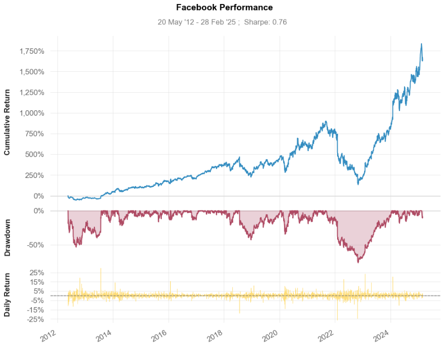
Seriesを渡せば問題なく動作しました。
では次にレポートを出力してみます。
qs.reports.html(stock['META'])
先ほどと同様、引数にはSeriesを渡さなければエラーとなります。また、Githubでは、2つ目の引数'SPY'を渡していますが、これもエラーが発生しました。SPYはベンチマークだと思いますが、これは省略しても動作します。ベンチマークを含めたレポートを出力したいときは下記のように別途データを取得すれば動作しました。
benchmark = qs.utils.download_returns('SPY')
qs.reports.html(stock['META'], benchmark['SPY'])
JupyterNotebookで実行したところ出力結果はHTMLファイルとしてダウンロードされました。

動作の詳細
各種統計の計算方法を知るためにGithubでコードを見ていきましょう。
sharpeを定義しているところを見てみると
def sharpe(returns, rf=0.0, periods=252, annualize=True, smart=False):
    """
    Calculates the sharpe ratio of access returns

    If rf is non-zero, you must specify periods.
    In this case, rf is assumed to be expressed in yearly (annualized) terms

    Args:
        * returns (Series, DataFrame): Input return series
        * rf (float): Risk-free rate expressed as a yearly (annualized) return
        * periods (int): Freq. of returns (252/365 for daily, 12 for monthly)
        * annualize: return annualize sharpe?
        * smart: return smart sharpe ratio
    """
    if rf != 0 and periods is None:
        raise Exception("Must provide periods if rf != 0")

    returns = _utils._prepare_returns(returns, rf, periods)
    divisor = returns.std(ddof=1)
    if smart:
        # penalize sharpe with auto correlation
        divisor = divisor * autocorr_penalty(returns)
    res = returns.mean() / divisor

    if annualize:
        return res * _np.sqrt(1 if periods is None else periods)

    return res
sharpe内で使われているリターン(シャープレシオの分子)については_utils._prepare_returnsの定義を確認する必要があります。
def _prepare_returns(data, rf=0.0, nperiods=None):
    """Converts price data into returns + cleanup"""
    data = data.copy()
    function = inspect.stack()[1][3]
    if isinstance(data, _pd.DataFrame):
        for col in data.columns:
            if data[col].dropna().min() >= 0 and data[col].dropna().max() > 1:
                data[col] = data[col].pct_change()
    elif data.min() >= 0 and data.max() > 1:
        data = data.pct_change()

    # cleanup data
    data = data.replace([_np.inf, -_np.inf], float("NaN"))

    if isinstance(data, (_pd.DataFrame, _pd.Series)):
        data = data.fillna(0).replace([_np.inf, -_np.inf], float("NaN"))
    unnecessary_function_calls = [
        "_prepare_benchmark",
        "cagr",
        "gain_to_pain_ratio",
        "rolling_volatility",
    ]

    if function not in unnecessary_function_calls:
        if rf > 0:
            return to_excess_returns(data, rf, nperiods)

    data = data.tz_localize(None)
    return data
_prepare_returnsはシャープレシオ以外にもいろいろと使われている前処理のようですね。インプットされたデータが終値なのかリターンなのかを判定して、リターンに統一しています。マイナスの数値が含まれる終値を入力するときなどには注意が必要かもしれないですね。(めったにないと思いますが。)

_prepare_returnsを直接呼び出して動作確認してみます。nan, inf, -infはそれぞれ0に置き換わり、リスクフリーレート分を調整しています。
シャープレシオの計算に戻ると
    res = returns.mean() / divisor

    if annualize:
        return res * _np.sqrt(1 if periods is None else periods)

    return res
となって、すでにreturnsにリスクフリーレートが反映済みということになります。
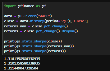
データをyfinanceで取得して、終値、株価リターン(欠損値そのまま)、株価リターン(欠損値削除)の3つで動作させてみると、株価リターン(欠損値削除)だけわずかに誤差が出ますね。終値を入れると内部でNaNが発生し、株価リターン(欠損値そのまま)と同じデータができて、それを処理されるわけです。
他の指標も使ってみる
ここからは個人的に気になったものをいくつかピックアップしてみます。
qs.statsにはgreeksというものも用意されています。
def greeks(returns, benchmark, periods=252.0, prepare_returns=True):
    """Calculates alpha and beta of the portfolio"""
    # ----------------------------
    # data cleanup
    if prepare_returns:
        returns = _utils._prepare_returns(returns)
    benchmark = _utils._prepare_benchmark(benchmark, returns.index)
    # ----------------------------

    # find covariance
    matrix = _np.cov(returns, benchmark)
    beta = matrix[0, 1] / matrix[1, 1]

    # calculates measures now
    alpha = returns.mean() - beta * benchmark.mean()
    alpha = alpha * periods

    return _pd.Series(
        {
            "beta": beta,
            "alpha": alpha,
            # "vol": _np.sqrt(matrix[0, 0]) * _np.sqrt(periods)
        }
    ).fillna(0)
オプションも対応してるのかと思いきや、アルファとベータを同時に計算するものでしたね。_prepare_returnsをあえてしない選択肢も用意されているみたいです。

次にrolling_greeks
def rolling_greeks(returns, benchmark, periods=252, prepare_returns=True):
    """Calculates rolling alpha and beta of the portfolio"""
    if prepare_returns:
        returns = _utils._prepare_returns(returns)
    df = _pd.DataFrame(
        data={
            "returns": returns,
            "benchmark": _utils._prepare_benchmark(benchmark, returns.index),
        }
    )
    df = df.fillna(0)
    corr = df.rolling(int(periods)).corr().unstack()["returns"]["benchmark"]
    std = df.rolling(int(periods)).std()
    beta = corr * std["returns"] / std["benchmark"]

    alpha = df["returns"].mean() - beta * df["benchmark"].mean()

    # alpha = alpha * periods
    return _pd.DataFrame(index=returns.index, data={"beta": beta, "alpha": alpha})
注意がいるのは引数のperiodsで、greeksではアルファの年率換算に使っているのに対して、rolling_greeksではローリングウインドウの期間になっていることでしょうか。

続いてドローダウンに関するところでdrawdown_detailsを見ていきます。
def to_drawdown_series(returns):
    """Convert returns series to drawdown series"""
    prices = _utils._prepare_prices(returns)
    dd = prices / _np.maximum.accumulate(prices) - 1.0
    return dd.replace([_np.inf, -_np.inf, -0], 0)


def drawdown_details(drawdown):
    """
    Calculates drawdown details, including start/end/valley dates,
    duration, max drawdown and max dd for 99% of the dd period
    for every drawdown period
    """

    def _drawdown_details(drawdown):
        # mark no drawdown
        no_dd = drawdown == 0

        # extract dd start dates, first date of the drawdown
        starts = ~no_dd & no_dd.shift(1)
        starts = list(starts[starts.values].index)

        # extract end dates, last date of the drawdown
        ends = no_dd & (~no_dd).shift(1)
        ends = ends.shift(-1, fill_value=False)
        ends = list(ends[ends.values].index)

        # no drawdown :)
        if not starts:
            return _pd.DataFrame(
                index=[],
                columns=(
                    "start",
                    "valley",
                    "end",
                    "days",
                    "max drawdown",
                    "99% max drawdown",
                ),
            )

        # drawdown series begins in a drawdown
        if ends and starts[0] > ends[0]:
            starts.insert(0, drawdown.index[0])

        # series ends in a drawdown fill with last date
        if not ends or starts[-1] > ends[-1]:
            ends.append(drawdown.index[-1])

        # build dataframe from results
        data = []
        for i, _ in enumerate(starts):
            dd = drawdown[starts[i] : ends[i]]
            clean_dd = -remove_outliers(-dd, 0.99)
            data.append(
                (
                    starts[i],
                    dd.idxmin(),
                    ends[i],
                    (ends[i] - starts[i]).days + 1,
                    dd.min() * 100,
                    clean_dd.min() * 100,
                )
            )

        df = _pd.DataFrame(
            data=data,
            columns=(
                "start",
                "valley",
                "end",
                "days",
                "max drawdown",
                "99% max drawdown",
            ),
        )
        df["days"] = df["days"].astype(int)
        df["max drawdown"] = df["max drawdown"].astype(float)
        df["99% max drawdown"] = df["99% max drawdown"].astype(float)

        df["start"] = df["start"].dt.strftime("%Y-%m-%d")
        df["end"] = df["end"].dt.strftime("%Y-%m-%d")
        df["valley"] = df["valley"].dt.strftime("%Y-%m-%d")

        return df

    if isinstance(drawdown, _pd.DataFrame):
        _dfs = {}
        for col in drawdown.columns:
            _dfs[col] = _drawdown_details(drawdown[col])
        return _pd.concat(_dfs, axis=1)

    return _drawdown_details(drawdown)
99% max drawdownは最大ドローダウン(および外れ値)の次に大きなドローダウンです。

詳細な情報がデータフレームとして返ってきます。
ソルティノレシオを確認します。
def sortino(returns, rf=0, periods=252, annualize=True, smart=False):
    """
    Calculates the sortino ratio of access returns

    If rf is non-zero, you must specify periods.
    In this case, rf is assumed to be expressed in yearly (annualized) terms

    Calculation is based on this paper by Red Rock Capital
    http://www.redrockcapital.com/Sortino__A__Sharper__Ratio_Red_Rock_Capital.pdf
    """
    if rf != 0 and periods is None:
        raise Exception("Must provide periods if rf != 0")

    returns = _utils._prepare_returns(returns, rf, periods)

    downside = _np.sqrt((returns[returns < 0] ** 2).sum() / len(returns))

    if smart:
        # penalize sortino with auto correlation
        downside = downside * autocorr_penalty(returns)

    res = returns.mean() / downside

    if annualize:
        return res * _np.sqrt(1 if periods is None else periods)

    return res
ソルティノレシオはリスクを下方偏差としていますが、下方偏差の厳密な計算方法がわかりにくかったりしますよね(?)
$$
\sigma_{\text{downside}} = \sqrt{\frac{\sum_{t=1}^{n} \min(R_t, 0)^2}{n}}
$$
Quantstatsではこのように定義していることがわかります。