はじめに
現在、中学受験はインターネットを背景としたデジタル化の加速により、スピード感を増しながら複雑化が進んでいます。これにより、教育現場では、専門的な知識と高い指導力を兼ね備えた人財の安定的な確保がますます困難な状況となっています。
中でも、「鶴亀算」に象徴される特殊算は、教える側の経験や属人的なノウハウに大きく依存しており、教育の標準化や持続可能な学習設計を阻む大きな障壁となっています。
特殊算は視覚的な発想に頼りがちで、形式的なパターン記憶に偏る傾向が強く、深い理解や応用力の育成には限界があると指摘されています。
そこで私たちは、鶴亀算の本質的な構造を、図解やモデルで体系化・可視化し、線形代数学の概念と接続する新たなアプローチへと進化させました。Pythonによるデジタル実装を通して、保護者様とお子様に寄り添う「ライフスタイル×学びのDX」を支援していきます。
参考リンク・動画
Python + Google Colab を活用したアジャイルな解法
私たちが提案する「つるがめソリューション」は、PythonとGoogle Colabを活用することで、従来の静的な問題演習とは異なるアジャイルで双方向的な学習体験を実現します。
Google Colabを使えば、保護者様やお子様が自らコードを実行し、数値を変更しながら、図を描き、検算し、数学的構造を実感として捉えることができます。
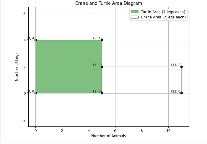
ソリューション1:お子様に面積で寄り添うつるがめソリューション
import numpy as np
import matplotlib.pyplot as plt

# 合計の個体数と足の数(つるかめ算)
A = 11  # 合計匹数 / Total number of animals
B = 32  # 合計足数 / Total number of legs

# ----------------------------
# 入力内容の表示 / Print input info
# ----------------------------
print("=== 入力 / Input ===")
print(f"合計の動物の数 A = {A} 匹")
print(f"合計の足の数 B = {B} 本")

# ----------------------------
# 連立方程式を解く(x: 亀の数, y: 鶴の数)
# ----------------------------
coeff_matrix = np.array([[1, 1],
                         [4, 2]])
constants = np.array([A, B])

x, y = np.linalg.solve(coeff_matrix, constants)

# ----------------------------
# 解の表示と検算(連立方程式)
# ----------------------------
print("\n=== 連立方程式の解 / Solution ===")
print(f"亀の数 (x) = {x}")
print(f"鶴の数 (y) = {y}")

# 検算 / Verification
check1 = x + y
check2 = 4 * x + 2 * y

print("\n=== 連立方程式の検算 / Verification ===")
print(f"x + y = {x} + {y} = {check1} → {'OK' if np.isclose(check1, A) else 'NG'} (期待値: {A})")
print(f"4x + 2y = 4×{x} + 2×{y} = {check2} → {'OK' if np.isclose(check2, B) else 'NG'} (期待値: {B})")

# ----------------------------
# 面積を使った考え方
# ----------------------------
area_4A = 4 * A                  # 全員が亀なら足の合計は 4 × A
diff_area = area_4A - B         # 差 = 余分な足の本数
diff_legs = 4 - 2               # 亀と鶴の足の差
num_cranes_by_area = diff_area / diff_legs
num_turtles_by_area = A - num_cranes_by_area

print("\n=== 面積を使った考え方 / Area-based Reasoning ===")
print(f"全員が亀なら足は 4 × {A} = {area_4A} 本")
print(f"実際の足の数との差: {area_4A} - {B} = {diff_area} 本")
print(f"1匹あたりの差(亀-鶴)= {diff_legs} 本")
print(f"差 ÷ 2 = {diff_area} ÷ {diff_legs} = {num_cranes_by_area} → 鶴の数")
print(f"A - 鶴の数 = {A} - {num_cranes_by_area} = {num_turtles_by_area} → 亀の数")

print("\n=== 面積から求めた面積値 / Area-based Foot Counts ===")
print(f"緑の面積(4×x)= {4 * x}")
print(f"白の面積(2×y)= {2 * y}")

# ----------------------------
# 検算(面積から)
# ----------------------------
print("\n=== 面積法による検算 / Verification (Area-based) ===")
legs_total = 4 * num_turtles_by_area + 2 * num_cranes_by_area
print(f"計算した足の数: 4×{num_turtles_by_area} + 2×{num_cranes_by_area} = {legs_total} 本(期待値: {B})")

# ----------------------------
# プロット領域の作成
# ----------------------------
plt.figure(figsize=(8, 6))

# 亀の領域(緑)
points_turtle = [(0, 0), (x, 0), (x, 4), (0, 4)]
plt.fill(*zip(*points_turtle), color='green', alpha=0.5, label='Turtle Area (4 legs each)')

# 鶴の領域(白)
points_crane = [(x, 0), (x + y, 0), (x + y, 2), (x, 2)]
plt.fill(*zip(*points_crane), color='white', edgecolor='black', label='Crane Area (2 legs each)')

# 点とラベルの描画
for point in points_turtle + points_crane:
    plt.scatter(*point, color='black')
    plt.text(point[0], point[1], f'({point[0]:.0f}, {point[1]:.0f})',
             fontsize=9, ha='right', va='bottom', color='black')

# 軸・タイトル・グリッド
plt.xlabel('Number of Animals')
plt.ylabel('Number of Legs')
plt.title('Crane and Turtle Area Diagram')
plt.legend()
plt.grid(True)
plt.axis('equal')
plt.show()
結果
=== 入力 / Input ===
合計の動物の数 A = 11 匹
合計の足の数 B = 32 本
=== 連立方程式の解 / Solution ===
亀の数 (x) = 5.0
鶴の数 (y) = 6.0
=== 連立方程式の検算 / Verification ===
x + y = 5.0 + 6.0 = 11.0 → OK (期待値: 11)
4x + 2y = 4×5.0 + 2×6.0 = 32.0 → OK (期待値: 32)
=== 面積を使った考え方 / Area-based Reasoning ===
全員が亀なら足は 4 × 11 = 44 本
実際の足の数との差: 44 - 32 = 12 本
1匹あたりの差(亀-鶴)= 2 本
差 ÷ 2 = 12 ÷ 2 = 6.0 → 鶴の数
A - 鶴の数 = 11 - 6.0 = 5.0 → 亀の数
=== 面積から求めた面積値 / Area-based Foot Counts ===
緑の面積(4×x)= 20.0
白の面積(2×y)= 12.0
=== 面積法による検算 / Verification (Area-based) ===
計算した足の数: 4×5.0 + 2×6.0 = 32.0 本(期待値: 32)
ソリューション2:アダルトな線形代数学ソリューション
import numpy as np
import matplotlib.pyplot as plt
from scipy.linalg import lu, solve_triangular

# 合計の動物の数と足の数(つるかめ算の例)
# Total number of animals and total number of legs
A = 11  # 匹 / animals
B = 32  # 本 / legs

# 連立方程式:
# Equation 1: x + y = A
# Equation 2: 4x + 2y = B

# 係数行列と定数ベクトルの定義 / Define coefficient matrix and constants vector
coeff_matrix = np.array([[1, 1],
                         [4, 2]])
constants = np.array([A, B])

# 1. NumPyで解く / Solve using NumPy
x_np, y_np = np.linalg.solve(coeff_matrix, constants)

# 2. クラメルの公式 / Cramer's Rule
det_main = np.linalg.det(coeff_matrix)
matrix_x = coeff_matrix.copy()
matrix_y = coeff_matrix.copy()
matrix_x[:, 0] = constants
matrix_y[:, 1] = constants
x_cramer = np.linalg.det(matrix_x) / det_main
y_cramer = np.linalg.det(matrix_y) / det_main

# 3. LU分解 / LU Decomposition
P, L, U = lu(coeff_matrix)
y_temp = solve_triangular(L, P @ constants, lower=True)
x_lu, y_lu = solve_triangular(U, y_temp)

# 4. QR分解 / QR Decomposition
Q, R = np.linalg.qr(coeff_matrix)
x_qr, y_qr = np.linalg.solve(R, Q.T @ constants)

# 5. 掃き出し法 / Gaussian Elimination
def gauss_elimination(A, b):
    A = A.astype(float)
    b = b.astype(float)
    n = len(b)
    Ab = np.hstack([A, b.reshape(-1, 1)])
    for i in range(n):
        Ab[i] = Ab[i] / Ab[i, i]
        for j in range(i + 1, n):
            Ab[j] = Ab[j] - Ab[j, i] * Ab[i]
    for i in range(n - 1, -1, -1):
        for j in range(i - 1, -1, -1):
            Ab[j] = Ab[j] - Ab[j, i] * Ab[i]
    return Ab[:, -1]

x_gauss, y_gauss = gauss_elimination(coeff_matrix, constants)

# 6. SVDによる擬似逆行列法 / Pseudo-inverse via SVD
x_svd = np.linalg.pinv(coeff_matrix) @ constants

# 7. 最小二乗法(過剰決定系も対応)/ Least Squares (for overdetermined systems)
x_ls, residuals, rank, s = np.linalg.lstsq(coeff_matrix, constants, rcond=None)

# 入力の表示 / Show input
print("=== 入力 / Input ===")
print(f"Total number of animals A = {A}")
print(f"Total number of legs B = {B}\n")

# 傾きと切片の表示 / Slopes and intercepts
slope1 = -1
intercept1 = A
slope2 = -2
intercept2 = B / 2

print("\n=== Slopes and Intercepts ===")
print(f"Line 1 (x + y = {A}): Slope = {slope1}, Intercept = {intercept1}")
print(f"Line 2 (4x + 2y = {B}): Slope = {slope2}, Intercept = {intercept2}")

# 各解法の結果を表示 / Display results
print("\n=== NumPy Solve ===")
print(f"x = {x_np}, y = {y_np}")

print("\n=== Cramer's Rule ===")
print(f"x = {x_cramer}, y = {y_cramer}")

print("\n=== LU Decomposition ===")
print(f"x = {x_lu}, y = {y_lu}")

print("\n=== QR Decomposition ===")
print(f"x = {x_qr}, y = {y_qr}")

print("\n=== Gaussian Elimination ===")
print(f"x = {x_gauss}, y = {y_gauss}")

print("\n=== Pseudo-inverse via SVD ===")
print(f"x = {x_svd[0]}, y = {x_svd[1]}")

print("\n=== Least Squares Method ===")
print(f"x = {x_ls[0]}, y = {x_ls[1]}")

# -----------------------------
# グラフ描画:直線の可視化 / Plot the two lines
# -----------------------------
x_vals = np.linspace(-5, 15, 200)
y1 = A - x_vals                 # y = -x + A
y2 = (B - 4 * x_vals) / 2       # y = -2x + B/2

plt.figure(figsize=(8, 6))
plt.plot(x_vals, y1, label='x + y = A', color='blue')
plt.plot(x_vals, y2, label='4x + 2y = B', color='green')
plt.plot(x_np, y_np, 'ro', label='Intersection (Solution)')
plt.xlabel('x (Turtles)')
plt.ylabel('y (Cranes)')
plt.title('Graphical Solution of the System')
plt.grid(True)
plt.legend()
plt.axhline(0, color='black', linewidth=0.5)
plt.axvline(0, color='black', linewidth=0.5)
plt.axis('equal')
plt.show()
結果
=== 入力 / Input ===
Total number of animals A = 11
Total number of legs B = 32
=== Slopes and Intercepts ===
Line 1 (x + y = 11): Slope = -1, Intercept = 11
Line 2 (4x + 2y = 32): Slope = -2, Intercept = 16.0
=== NumPy Solve ===
x = 5.0, y = 6.0
=== Cramer's Rule ===
x = 5.000000000000001, y = 6.0
=== LU Decomposition ===
x = 5.0, y = 6.0
=== QR Decomposition ===
x = 4.9999999999999964, y = 6.000000000000007
=== Gaussian Elimination ===
x = 5.0, y = 6.0
=== Pseudo-inverse via SVD ===
x = 4.999999999999994, y = 6.00000000000001
=== Least Squares Method ===
x = 4.999999999999996, y = 6.000000000000007

まとめ
コードの細かな解説は割愛します。なぜなら、私たちはアジャイルなプロンプトエンジニアリングという対話型AIとの学びを大切にしているからです。
コードをコピペして動かし、グラフを眺めて、あなた自身の問いと仮説に基づいて試行錯誤してください。そうしたプロセスこそが、学びを深め、直感と論理の両輪を育ててくれるでしょう。
参考動画:
鶴亀算は、特殊算と連立方程式、そして線形代数学をつなぐ “ソリューションズ” です。
教育課題DX、学習者のつまずき、そして数学の楽しさの再発見。
社会のお困りに対して、アジャイルなソリューションで共に成長を加速していきましょう。