はじめに:中学受験を取り巻く変化と課題
近年、中学受験を巡る教育環境は大きく変化しています。オンライン教材、デジタル学習管理ツールなどが普及し、学びは「紙」から「デバイス」へと大きくシフトしています。一方で、教科横断的な理解が求められる中、「音の高さ」や「振動数」といった理科と算数の融合的テーマは、指導する教育職人さんの専門性や経験値に大きく依存しており、標準化・持続可能な教育の障壁となっています。
本質的な理解に必要なのは「体験による感動」
音の高さを理解するうえで、最も重要なのは公式の暗記ではなく、耳と目と心での体験です。たとえば以下のような問いを投げかけたとき、子どもはどのように学ぶでしょうか?
「弦の長さが2倍になると、音はどう変わると思う?」
「おもりの数が増えると、音は高くなる?低くなる?」
こうした質問に対し、数式で説明する前に“聴いて感じる”ことができれば、抽象的な振動数や周期の概念も直感的に理解できます。
ソリューション:Python + Google Colabによる「音の見える化」
私たちのソリューションは、PythonコードとGoogle Colaboratoryを活用し、音の原理を「再生」「視覚化」「数式化」できるよう設計された学習教材です。以下の技術的要素を含みます:
技術構成(Pythonによる体験設計)
-
振動数の定義式:
( f = \frac{k \cdot \sqrt{N}}{L \cdot T} ) に基づく音の周波数モデル - 弦の太さ・長さ・おもりの数をパラメータに持つ
- 振動数(周波数)に基づくサイン波の生成と可視化
- 1周期と2秒間の波形表示による音の高さの違いの理解
- 実際の音声としての再生(Google Colab上で実行)
Google Colab導入のリンク例:
🔗 実演動画はこちら
実行してみよう:Google Colabに貼り付けて実行可能
pip install ipython
import math # 平方根 (sqrt) を計算するため / For square root (sqrt) calculation
import numpy as np # サイン波の計算に必要 / For sine wave computation
import matplotlib.pyplot as plt # プロットのために必要 / For plotting
from IPython.display import Audio, display # Google Colabで音を再生 / For audio playback in Google Colab
# 1. 初期条件を定義 / Define initial conditions
initial_thickness = 0.1 # 初期の太さ (仮定単位: cm) / Initial thickness (assumed unit: cm)
initial_length = 10 # 初期の長さ (cm) / Initial length (cm)
initial_weight_count = 1 # 初期のおもりの個数 / Initial number of weights
initial_frequency = 200 # 初期の振動数 (Hz) / Initial frequency (Hz)
# 2. 比例定数 k を計算 / Calculate the proportionality constant k
# f = k * sqrt(N) / (L * T) より、k = f * (L * T) / sqrt(N)
# From f = k * sqrt(N) / (L * T), k = f * (L * T) / sqrt(N)
k = initial_frequency * (initial_length * initial_thickness) / math.sqrt(initial_weight_count)
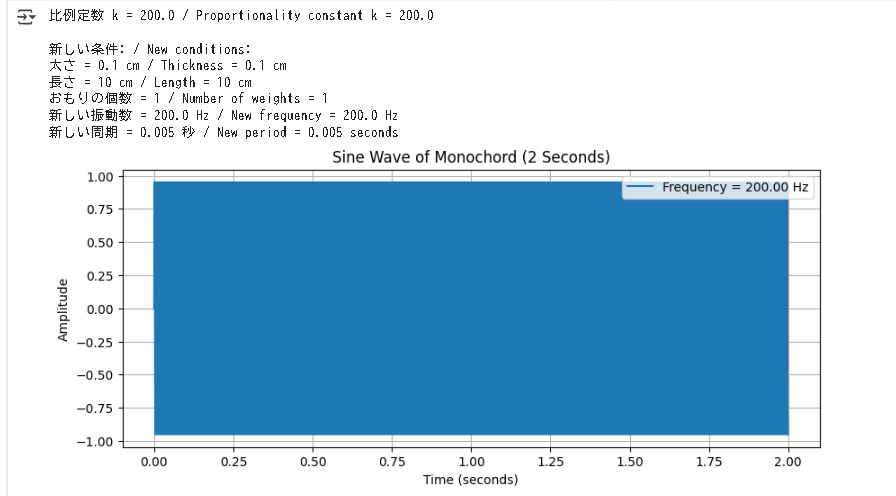
print(f"比例定数 k = {k} / Proportionality constant k = {k}")
# 3. 新しい条件を定義 / Define new conditions
new_thickness = 0.1 # 新しい太さ (cm) / New thickness (cm)
new_length = 10 # 新しい長さ (cm) / New length (cm)
new_weight_count = 1 # 新しいおもりの個数 / New number of weights
# 新しい条件を表示 / Display new conditions
print("\n新しい条件: / New conditions:")
print(f"太さ = {new_thickness} cm / Thickness = {new_thickness} cm")
print(f"長さ = {new_length} cm / Length = {new_length} cm")
print(f"おもりの個数 = {new_weight_count} / Number of weights = {new_weight_count}")
# 4. 新しい振動数を計算 / Calculate new frequency
new_frequency = k * math.sqrt(new_weight_count) / (new_length * new_thickness)
print(f"新しい振動数 = {new_frequency} Hz / New frequency = {new_frequency} Hz")
# 5. 周期を計算 / Calculate period
# 周期 T = 1 / f / Period T = 1 / f
new_period = 1 / new_frequency
print(f"新しい周期 = {new_period} 秒 / New period = {new_period} seconds")
# 6. 2秒間のサイン波をプロット / Plot sine wave for 2 seconds
# 時間軸を定義 (0から2秒、0.001秒間隔) / Define time axis (0 to 2 seconds, 0.001-second intervals)
time_full = np.arange(0, 2, 0.001)
# サイン波: y = sin(2πft) / Sine wave: y = sin(2πft)
amplitude = 1 # 振幅(任意に1とする) / Amplitude (arbitrarily set to 1)
sine_wave_full = amplitude * np.sin(2 * np.pi * new_frequency * time_full)
# 2秒間のプロット設定 / Plot settings for full 2-second wave
plt.figure(figsize=(10, 4))
plt.plot(time_full, sine_wave_full, label=f'Frequency = {new_frequency:.2f} Hz')
plt.title("Sine Wave of Monochord (2 Seconds)")
plt.xlabel("Time (seconds)")
plt.ylabel("Amplitude")
plt.grid(True)
plt.legend()
plt.show()
# 7. 1周期のサイン波をプロット / Plot sine wave for one period
# 1周期の時間軸を定義 (0からT、0.0001秒間隔で高解像度) / Define time axis for one period (0 to T, 0.0001-second intervals for finer resolution)
time_one_period = np.arange(0, new_period, 0.0001)
sine_wave_one_period = amplitude * np.sin(2 * np.pi * new_frequency * time_one_period)
# 1周期のプロット設定 / Plot settings for one period
plt.figure(figsize=(10, 4))
plt.plot(time_one_period, sine_wave_one_period, label=f'Frequency = {new_frequency:.2f} Hz, Period = {new_period:.4f} s')
plt.title("Sine Wave of Monochord (One Period)")
plt.xlabel("Time (seconds)")
plt.ylabel("Amplitude")
plt.grid(True)
plt.legend()
plt.show()
# 8. Google Colabで音を再生 / Play sound in Google Colab
# サンプリングレートを定義(人間の可聴範囲に合わせて44100 Hz) / Define sample rate (44100 Hz for audible range)
sample_rate = 44100
# 5秒間の音声データを生成 / Generate 5 seconds of audio data
audio_time = np.arange(0, 5, 1/sample_rate)
audio_wave = amplitude * np.sin(2 * np.pi * new_frequency * audio_time)
# Audioオブジェクトを作成して再生 / Create and play Audio object
audio = Audio(audio_wave, rate=sample_rate)
display(audio)
Google Colabにアクセスし、Pythonコードを実行するだけで、音が「見える」「聞こえる」教材体験が実現できます。
結果
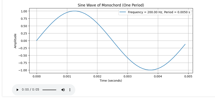
再生ボタンを押すと音が再生できます
おわりに:STEM教育の架け橋としての音体験DX
このソリューションは、算数・理科・プログラミングを融合した学びとして構築されています。
「感動を伴う体験が深い理解へと導く」という信念のもと、
コードの解説は、マルチモーダルな生成AIとのアジャイルな対話を通じて、成長を飛躍的に加速させましょう。
お子様が音と数式を探究することで、生活に根ざしたデジタルソリューションを自ら生み出せる未来を、心から願っています。