Handling Big Categorical Variables #R

Dealing with categorical variables in your data can be a nasty experience.

Categorical variables come in several forms: ordered, unordered, intervals, high cardinality and low cardinality. On top of that different algorithms handle categorical variables differently. As an example, random forest implementations can handle categorical variables without requiring to encode them into numerical values while regression models and binary boosted tree implementations (Xgboost) require them to be numerically encoded first. Further, there is a possibility that two categorical variables interact to form a more influential categorical variable. Thus n-way-interactions also need to be explored. Well then why miss numerical-categorical interactions?

To ease down this categorical mess, I discuss tips from my experience working on small and big data sets and several Kaggle competitions. I have tried to also incorporate some home-grown R functions I usually use to handle categorical variables.

So I provide a useful summary of handling categorical variables for different kinds of algorithms and data sizes. I gained this experience through analysing various data-sets and doing Kaggle competitions and thus also created my own home-grown functions I usually use in R.

Useful Encoding Systems

One-Hot / Dummy Encoding: Most commonly used. There are two types: full-rank and not-full-rank. The former gives $(C-1)$ output features for $C$ levels while the later gives $C$ output features. GLM models usually require full-rank encodings while tree-based algorithms can handle and benefit from non-full-rank encodings. However, one-hot encoding become quite memory intensive for high cardinality variables like zip_code.

# Function for one-hot-encoding
# data must contain all character/factor columns needed to be encoded.
categtoOnehot <- function(data, fullrank=T, ...){
  data[,names(data)] = lapply(data[,names(data)] , factor) # convert character to factors
  if (fullrank){
    res = as.data.frame(as.matrix(model.matrix( ~., data, ...)))[,-1]
  } else {
    res = as.data.frame(as.matrix(model.matrix(~ ., data, contrasts.arg = lapply(data, contrasts, contrasts=FALSE), ...)))[,-1]
  }
return(res)
}

# example
dd <- read.table(text="
   RACE        AVG.AGE     INCOMEGROUP
                 HISPANIC          41          M
                 ASIAN             45          H
                 HISPANIC          39          L
                 CAUCASIAN         40          M",
                 header=TRUE)


categtoOnehot(dd[,c(1,3)], fullrank=T)
#  RACECAUCASIAN RACEHISPANIC INCOMEGROUPL INCOMEGROUPM
#1             0            1            0            1
#2             0            0            0            0
#3             0            1            1            0
#4             1            0            0            1


categtoOnehot(dd[,c(1,3)], fullrank=F)
#  RACEASIAN RACECAUCASIAN RACEHISPANIC INCOMEGROUPH INCOMEGROUPL INCOMEGROUPM
#1         0             0            1            0            0            1
#2         1             0            0            1            0            0
#3         0             0            1            0            1            0
#4         0             1            0            0            0            1

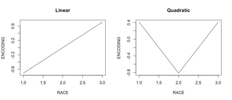
Orthogonal Polynomial encoding: Mostly used for ordered categorical variables (ex. INCOMEGROUP). The encodings are given by coefficients of linear, quadratic, cubic (and so on) polynomials orthogonal to each other. One major benefit is that it can be used to identify quadratic/cubic/ etc. relationships of the variable with the target. However many of them may turn out to be noise and must be eliminated.

# Function for Orthogonal-Polynomial-Encoding
categtoOrthPoly <- function(data, ...){
  data[,names(data)] = lapply(data[,names(data)] , ordered) # convert character to factors
  res = as.data.frame(as.matrix(model.matrix( ~., data, ...)))[,-1]
  return(res)
}

# example
categtoOrthPoly(dd[,c(1,3)])
#         RACE.L     RACE.Q INCOMEGROUP.L INCOMEGROUP.Q
#1  7.071068e-01  0.4082483  7.071068e-01     0.4082483
#2 -7.071068e-01  0.4082483 -7.071068e-01     0.4082483
#3  7.071068e-01  0.4082483 -7.850462e-17    -0.8164966
#4 -7.850462e-17 -0.8164966  7.071068e-01     0.4082483

The following figure shows plots of Linear and Quadratic Encodings of variable Race.

Deviation Encoding: Mostly used for high cardinality variables. Technically it refers to deviation of mean of target of one level from the mean of mean of targets of all levels. For example if means of target for levels-1,2,3,4 are 31.24, 41.56, 53.23, 22.34 then level 1 will be encoded as $\frac{31.24 \ + \ 41.56 \ + \ 53.23 \ + \ 22.34}{4}$ - 31.24 = 5.8525. But we can generalise it to replace target by other numerical features and mean by median/sd or other statistical measures. Note that these encodings must be created out-of-fold using only training data values because target is not observed for test data.

# Function to create mean/sd/median deviation encoding w.r.t to numerical features
require(dplyr)
categtoDeviationenc <- function(char_data, num_data, traininds=NULL, funcs = funs(mean(.,na.rm=T), sd(.,na.rm=T), 'median' = median(.,na.rm=T))){

  if(length(traininds) == 0){
    train_char_data = char_data
    train_num_data = num_data
  } else {
    train_char_data = char_data[traininds, ]
    train_num_data =num_data[traininds, ]
  }

  res = list()
  for(x in names(train_char_data)){
    res[[x]] = train_num_data %>% group_by(.dots=train_char_data[,x]) %>% summarise_each(funcs) # calculate mean/sd/median encodings
    res[[x]][,-1] = apply(res[[x]][,-1], 2, scale, scale=FALSE, center=TRUE) # calculate deviances of mean/sd/median encodings
    # rename columns
    colnames(res[[x]])[1] = x 
    if (ncol(train_num_data) == 1)
      colnames(res[[x]])[-1] = paste0(names(train_num_data),'_',names(res[[x]])[-1])
    res[[x]] <- merge(char_data[,x,drop=F], res[[x]], all.x=T, by=x)[,-1] # apply encodings to all data
  }
  res = data.frame(do.call(cbind, res))
  return(res)
}

# example
categtoDeviationenc(char_data = dd[,c(1,3)], num_data = dd[,2,drop=F])
#  RACE.AVG.AGE_mean RACE.AVG.AGE_sd RACE.AVG.AGE_median INCOMEGROUP.AVG.AGE_mean INCOMEGROUP.AVG.AGE_sd INCOMEGROUP.AVG.AGE_median
#1          3.333333              NA            3.333333                      3.5                     NA                        3.5
#2         -1.666667              NA           -1.666667                     -2.5                     NA                       -2.5
#3         -1.666667               0           -1.666667                     -1.0                      0                       -1.0
#4         -1.666667               0           -1.666667                     -1.0                      0                       -1.0

Other encodings: There are other systems of encodings like Helmert, Reverse Helmert, Forward Difference, Backward difference which are summarised here but are seldom used. Encodings may also be user defined using contrast matrices as described in the same link.

A Summary of Encodings

Encoding	Type of cat var	Cardinality Suited for	Algorithms Suited for
Raw	any	any	Tree-based algorithms that can handle category splits internally (RF)
One-hot Encoding	any	low-medium	Xgboost, GLM
Orthogonal Polynomial Encoding	ordered, interval	low	Xgboost, RF, GLM
Deviance Encoding	any	medium-high	Xgboost, RF, GLM

Exploring Feature Interactions

There can be two types of categorical feature interactions:

Categorical-Categorical Interactions: Given, m categorical variables, there are in general $m \choose n$ n-way-interactions that can be created but several of these are equivalent to other categorical variables and thus need to be filtered out. Depending on their cardinality size, ordered/unordered and algorithm used they can be encoded using above techniques.

# Function to remove equivalent factors
remEquivfactors <- function(x.data, ref.data = NULL){
  if(length(ref.data) == 0L){
    all = x.data
  } else{
    all = data.frame(cbind(ref.data, x.data))
  }
  all[,names(all)] = lapply(all[,names(all), drop=F], function(l){
    as.numeric(reorder(x=l, X=seq(1:nrow(all)), FUN=mean))
  })
  rem = which(!(names(x.data) %in% colnames(unique(as.matrix(all), MARGIN=2, fromLast = F)))) # removal of cols towards end will be preferred
  return(rem)
}

# Function to create n-way categorical-categorical interactions
nwayInterac <- function(char_data, n){
  nway <- as.data.frame(combn(ncol(char_data), n, function(y) do.call(paste0, char_data[,y])))
  names(nway) = combn(ncol(char_data), n, function(y) paste0(names(char_data)[y], collapse='.'))
  rem = remEquivfactors(x.data = nway, ref.data=NULL)
  if(length(rem) > 0)
    nway = nway[,-rem]
  return(nway)
}

# example
nwayInterac(dd[,c(1,3)], n=2)
#  RACE.INCOMEGROUP
#1        HISPANICM
#2           ASIANH
#3        HISPANICL
#4       CAUCASIANM

Categorical-Numerical Interactions: These can be formed by multiplying a numerical feature by an encoded categorical feature. Usually numerical features are multiplied by one-hot-encoded categorical features because such interactions are easy to interpret intuitively.

The space of n-way-interactions can grow very fast with increasing cardinalities. A lot of interactions may just be noise. Thus interactions must be chosen carefully and noise eliminated regularly. Here are some tips that can be followed for doing so:

For large $n$, choose interaction randomly and test using a simple linear model to throw away noisy/meaningless interactions.
For high cardinality interactions, use deviation encodings.
Explore model dumps of tree-based algorithms like Xgboost and Random Forests to find useful deep interactions. For Xgboost, xgbfi is a useful tool to explore feature interactions by different metrics.
Always keep track of equivalent categorical variables or identical/highly correlated features to manage data size.
Keep note of the fact that Random forests feature importance is usually biased towards high cardinality features and numerical features.
Glmnet is a good linear model to filter out noisy interactions.
Forward feature selection using a linear model can be used to rank importance of categorical features and interactions.

You can find my gist of useful feature engineering functions here.