ディープラーニング入門: 手書き文字認識

入門者向け：Pythonでニューラルネットワークを使った手書き文字認識

ニューラルネットワークは、近年、さまざまな分野で広く使われている技術の一つです。特に、画像認識のタスクでは、その能力を最大限に発揮します。この記事では、手書き文字認識の問題を通じて、シンプルなニューラルネットワークである「多層パーセプトロン（MLP）」を使った実装方法を解説します。

1. ニューラルネットワークの基本

ニューラルネットワークは、人間の脳の神経回路に触発されたアルゴリズムです。複数の層を通してデータを処理し、特定のタスク（分類や予測など）を実行します。ニューラルネットワークにはさまざまな種類がありますが、今回はその中でもシンプルな 多層パーセプトロン（MLP: multi-layer perceptron） を使用します。

2. 手書き文字認識とは

手書き文字認識は、画像から手書きの数字を読み取り、その数字を正しく分類するタスクです。今回使用するデータセットは、機械学習の入門でよく使用される「MNISTデータセット」です。このデータセットは28x28ピクセルの手書き数字画像を含んでおり、ニューラルネットワークの学習に最適です。

3. 実装手順

1. データ準備

まず、MNISTデータセットをロードし、データの形状や内容を確認します。

from tensorflow.keras.datasets import mnist

# データセットのロード
(x_train, y_train), (x_test, y_test) = mnist.load_data()

# データの形状を確認
print(f"x_train.shape = {x_train.shape}")
print(f"y_train.shape = {y_train.shape}")

このデータは28x28ピクセルのグレースケール画像ですが、ニューラルネットワークに入力するために1次元ベクトルに変換し、ピクセルの値を0から1の範囲に正規化します。

画像データの生データを確認します。

fig = plt.figure(figsize=(9, 15))
fig.subplots_adjust(left=0, right=1, bottom=0, top=0.5, hspace=0.05, wspace=0.05)
for i in range(9):
    ax = fig.add_subplot(1, 9, i + 1, xticks=[], yticks=[])
    ax.set_title(str(y_train[i]))
    ax.imshow(x_train[i], cmap='gray')

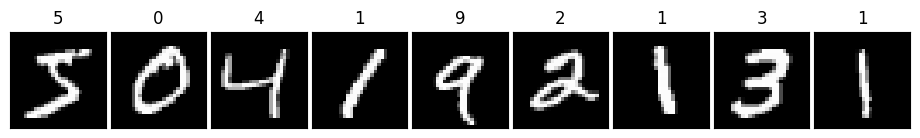
こんな感じで白黒の手書き文字が格納されています。

# 画像データを28x28から784のベクトルに変換
x_train = x_train.reshape(-1, 28*28).astype('float32') / 255.0
x_test = x_test.reshape(-1, 28*28).astype('float32') / 255.0

また、ラベル（数字）をOne-Hotエンコーディングという形式に変換し、分類タスクで使える形にします。

from tensorflow.keras.utils import to_categorical

y_train = to_categorical(y_train)
y_test = to_categorical(y_test)

2. モデル構築

次に、MLPのモデルを構築します。このモデルには3つの層があり、それぞれ異なる役割を持っています。

• 入力層: 手書き数字画像（784次元のベクトル）
• 中間層: 隠れ層で、256と100のユニットを持ち、ReLUという活性化関数を使用
• 出力層: 10クラス（0から9の数字）を分類するための出力層

from tensorflow.keras.models import Sequential
from tensorflow.keras.layers import Dense, Activation

model = Sequential()
model.add(Dense(units=256, input_shape=(28*28,)))
model.add(Activation('relu'))
model.add(Dense(units=100))
model.add(Activation('relu'))
model.add(Dense(units=10))
model.add(Activation('softmax'))

次に、モデルをコンパイルします。損失関数には交差エントロピー誤差を、最適化アルゴリズムには 確率的勾配降下法（SGD） を使用します。

model.compile(
    loss='categorical_crossentropy',
    optimizer='sgd',
    metrics=['accuracy']
)

参考として、モデル構造を可視化します。

### モデル構造の可視化
from tensorflow.keras.utils import plot_model
from IPython.display import Image, display

# モデルをPNGファイルとして保存
plot_model(
    model,
    to_file='model.png',
    show_shapes=True,
    show_layer_names=True,
    expand_nested=True,
    dpi=96,
    show_dtype=False
)

# 保存したPNGファイルを表示
display(Image(filename='model.png'))

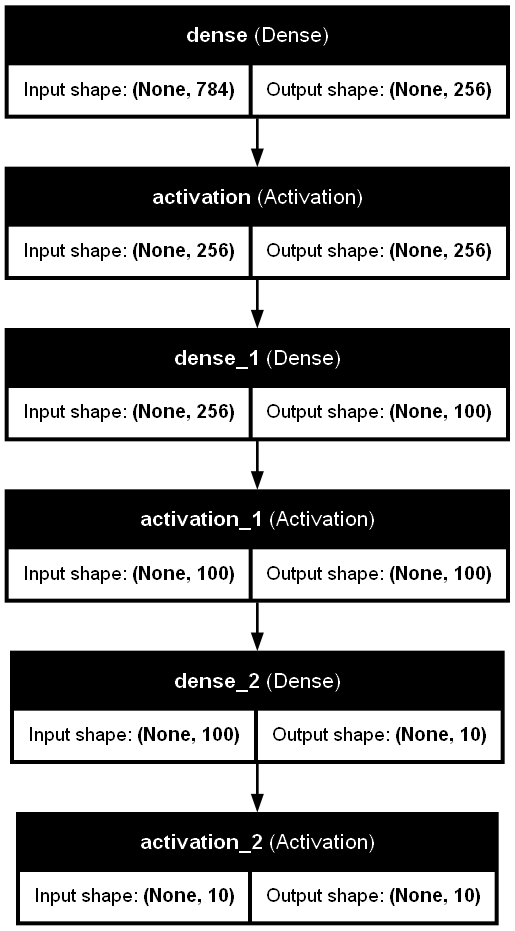
可視化されたモデル構造は以下の通りです。
入力層→活性化関数→全結合層→活性化関数→全結合層→活性化関数という構造になっています。

3. モデルの訓練と評価

モデルを構築したら、データを使って訓練します。訓練データでモデルを学習させ、テストデータでモデルの性能を評価します。

history = model.fit(
    x_train, y_train,
    epochs=10,
    batch_size=1000,
    validation_data=(x_test, y_test),
    verbose=1
)

訓練が終わったら、テストデータでの損失と精度を確認します。

test_loss, test_acc = model.evaluate(x_test, y_test, verbose=0)
print(f'テスト損失: {test_loss:.4f}')
print(f'テスト精度: {test_acc:.4f}')

4. 学習の進行状況の可視化

モデルの学習過程を視覚化することで、モデルがどのように学習しているのかを確認します。特に、損失と精度の変化をプロットすることで、過学習などの問題を発見できます。

import matplotlib.pyplot as plt

plt.figure(figsize=(12, 4))

# 損失のプロット
plt.subplot(1, 2, 1)
plt.plot(history.history['loss'], label='Train_loss')
plt.plot(history.history['val_loss'], label='Validation')
plt.title('Loss')
plt.xlabel('Epoch')
plt.ylabel('Loss')
plt.legend()

# 精度のプロット
plt.subplot(1, 2, 2)
plt.plot(history.history['accuracy'], label='Train')
plt.plot(history.history['val_accuracy'], label='Validation')
plt.title('Accuracy')
plt.xlabel('Epoch')
plt.ylabel('Accuracy')
plt.legend()

plt.show()

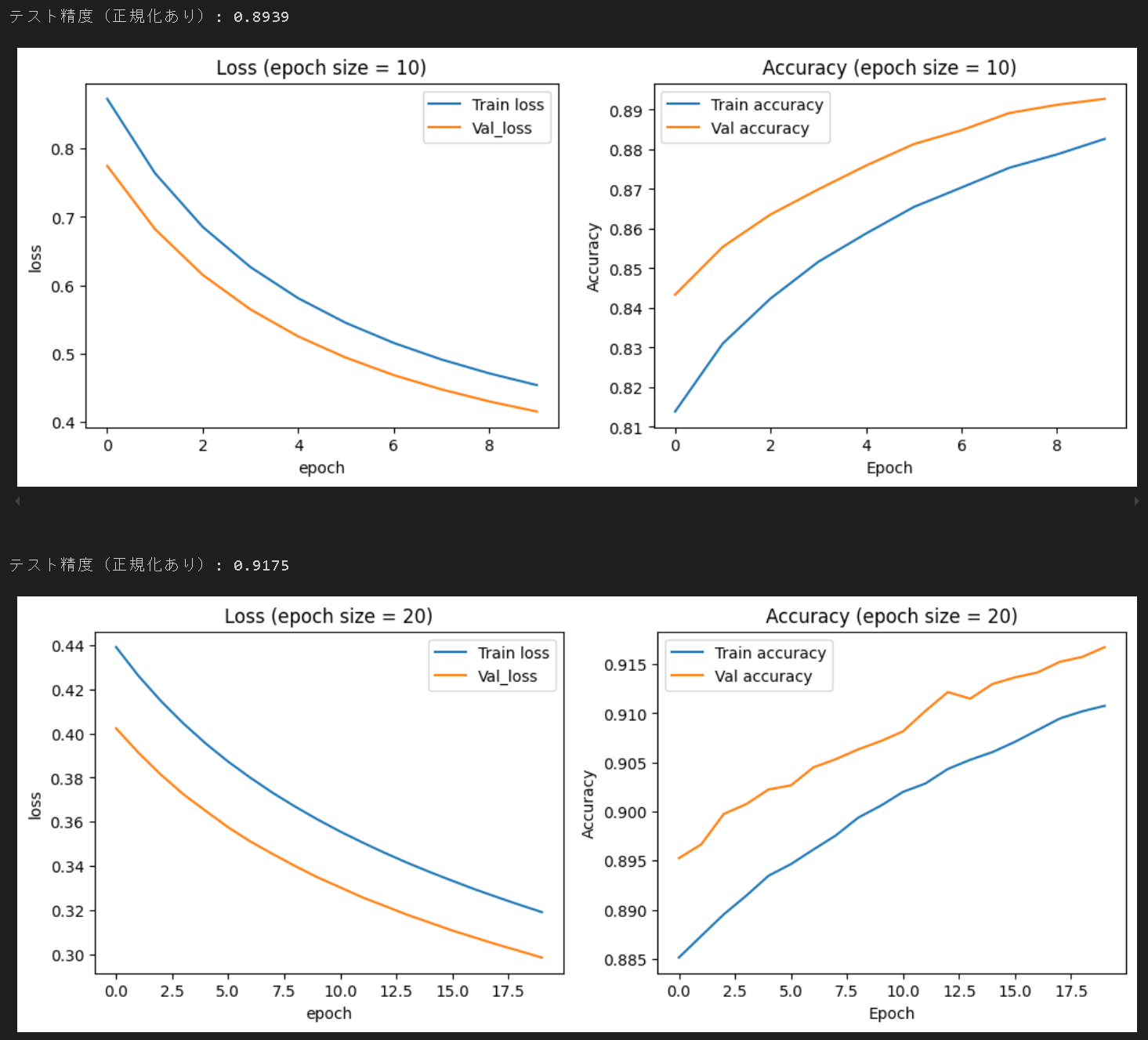
可視化した学習過程は以下の通りです。左のグラフから、学習が進むにほど（X軸のエポック数が増加するほど）、Lossが減少している（予測性能が向上している）ことが視認できます。右のグラフでは、学習が進むほど、Accuracyが増加し、学習初期は0.6程度あってたAccuracyが最終的には0.9足らずまで向上したことが分かります。

---

コード全文

# 必要なライブラリのインポート
import tensorflow as tf
from tensorflow import keras
from tensorflow.keras.datasets import mnist
import matplotlib.pyplot as plt
from tensorflow.keras.utils import to_categorical, plot_model
from tensorflow.keras.models import Sequential
from tensorflow.keras.layers import Dense, Activation
from typing import Tuple
import numpy as np

# 1. データ準備

# MNISTデータセットのロード
(x_train, y_train), (x_test, y_test) = mnist.load_data()

# データの形状を確認
print(f"x_train.shape = {x_train.shape}")
print(f"y_train.shape = {y_train.shape}")

# 手書き数字の画像を可視化
fig = plt.figure(figsize=(9, 15))
fig.subplots_adjust(left=0, right=1, bottom=0, top=0.5, hspace=0.05, wspace=0.05)
for i in range(9):
    ax = fig.add_subplot(1, 9, i + 1, xticks=[], yticks=[])
    ax.set_title(str(y_train[i]))
    ax.imshow(x_train[i], cmap='gray')
plt.show()

# データの前処理

# 画像データを28x28から784のベクトルに変換
x_train: np.ndarray = x_train.reshape(-1, 28*28)
x_test: np.ndarray = x_test.reshape(-1, 28*28)

# ピクセル値を0~1の範囲に正規化
x_train = x_train.astype('float32') / 255.0
x_test = x_test.astype('float32') / 255.0

# ラベルをOne-Hotベクトルに変換
y_train: np.ndarray = to_categorical(y_train)
y_test: np.ndarray = to_categorical(y_test)

# 2. モデル構築

# MLPモデルの定義
model: Sequential = Sequential()
model.add(Dense(units=256, input_shape=(28*28,)))  # 入力層
model.add(Activation('relu'))  # 活性化関数ReLU
model.add(Dense(units=100))  # 中間層
model.add(Activation('relu'))
model.add(Dense(units=10))  # 出力層
model.add(Activation('softmax'))  # 活性化関数Softmax

# モデルのコンパイル
model.compile(
    loss='categorical_crossentropy',  # 損失関数（交差エントロピー誤差）
    optimizer='sgd',  # 最適化アルゴリズム（確率的勾配降下法）
    metrics=['accuracy']  # 評価指標（正解率）
)

# 3. モデルの学習

# モデルの訓練
history = model.fit(
    x_train, y_train,
    epochs=10,
    batch_size=1000,
    validation_data=(x_test, y_test),
    verbose=1
)

# モデルの評価
test_loss, test_acc = model.evaluate(x_test, y_test, verbose=0)
print(f'\nテスト損失: {test_loss:.4f}')
print(f'テスト精度: {test_acc:.4f}')

# 4. 学習の進行状況の可視化

plt.figure(figsize=(12, 4))

# 損失のプロット
plt.subplot(1, 2, 1)
plt.plot(history.history['loss'], label='Train_loss')
plt.plot(history.history['val_loss'], label='Validation')
plt.title('Loss')
plt.xlabel('Epoch')
plt.ylabel('Loss')
plt.legend()

# 精度のプロット
plt.subplot(1, 2, 2)
plt.plot(history.history['accuracy'], label='Train')
plt.plot(history.history['val_accuracy'], label='Validation')
plt.title('Accuracy')
plt.xlabel('Epoch')
plt.ylabel('Accuracy')
plt.legend()

plt.show()

---

4. 学習条件が性能に与える影響

4.1. エポック数の影響

エポック数を10から20に増やすと、訓練終了時のロスが0.5程度から0.32程度まで減少し、Accuracyが0.89から0.91に増加している、つまり予測性能が向上していることが分かる。
エポック数、つまり学習回数を増加させると、性能が向上する傾向が確認できた。さらにエポック数を増加させると、訓練データに過剰にフィッティングする過学習のリスクも増大する点には注意が必要とのこと。

4.2. バッチサイズの影響

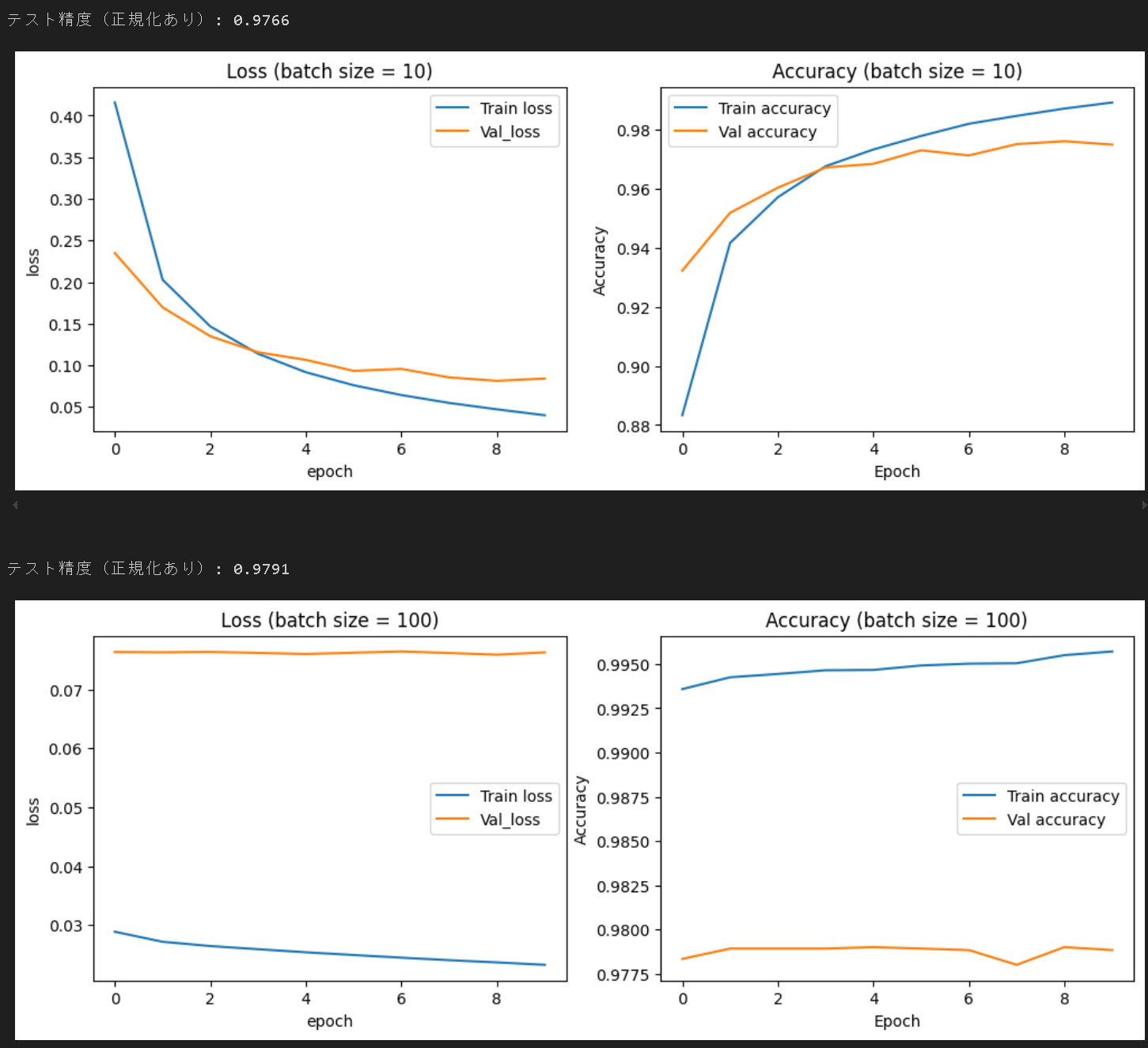
バッチサイズを10から100に10倍化した結果、Accuracyが0.976から0.979に若干増加した。若干性能が向上したものの、グラフをいると、訓練ロスと検証ロスの差が開いていることが分かり、同様の傾向がAccuracyでも確認できる。訓練ロスが検証ロスよりも小さいことから、訓練データに過学習している状態と考えられる。バッチサイズを不適切に設定するとモデル性能の劣化につながる恐れがあると考えられる。

4.3. モデル性能に影響する要素例:

• MLPのアーキテクチャの工夫:
  • 層の追加
  • ユニット数の変更
  • 活性化関数の追加、種類の変更
  • ドロップアウトの追加、割合の調整
  • 正則化の追加
• データ前処理の工夫:
  • データ正規化（例: ピクセル値を0~1に正則化）
  • データ拡張（例: 画像を回転させる、ズームする、シフトする）
• ハイパーパラメータのチューニング:
  • 学習率（大きいほど学習効率が向上するが、収束しない可能性もある）
    • 学習率スケジューリングの導入（学習の進捗に応じて学習率を調整する）
    • 学習率ウォームアップ（徐々に学習率を上げる）
  • バッチサイズ（大きいほど計算効率が向上するが、＊＊＊な可能性もある）
  • 最適化アルゴリズムの変更（Adam、SGD、RMSprop、Adagardなど様々なアルゴがある）
    • 勾配クリッピング（勾配の爆発を防止）
• MLP以外のアーキテクチャの使用:
  • CNNの使用
  • アンサンブル学習：複数モデルを組み合わせる

---

5. まとめ

今回の記事では、手書き文字認識の問題を通じて、シンプルなニューラルネットワーク（多層パーセプトロン、MLP）の基本的な実装を解説しました。ニューラルネットワークの構築から学習、そして評価と可視化までのフローを理解することで、画像認識タスクへのアプローチが一歩進みました。Kerasのような高レベルAPIを利用することで、想像していたより少ないコード量でニューラルネットワークを実装できることに驚きました。大量の訓練データを集めること、訓練データの前処理を工夫すること、モデルのアーキテクチャを工夫すること、学習条件を工夫すること、が主な差別化ポイントだと理解しました。特に、訓練データを集めることが一番難しく、データを持っていること自体が強み、になると感じました。

次のステップとして、 畳み込みニューラルネットワーク（CNN） を学習する予定です。