#Pythonで学ぶ制御工学< ディジタル実装 >
はじめに
基本的な制御工学をPythonで実装し,復習も兼ねて制御工学への理解をより深めることが目的である.
その第25弾として「ディジタル実装」を扱う.
概要
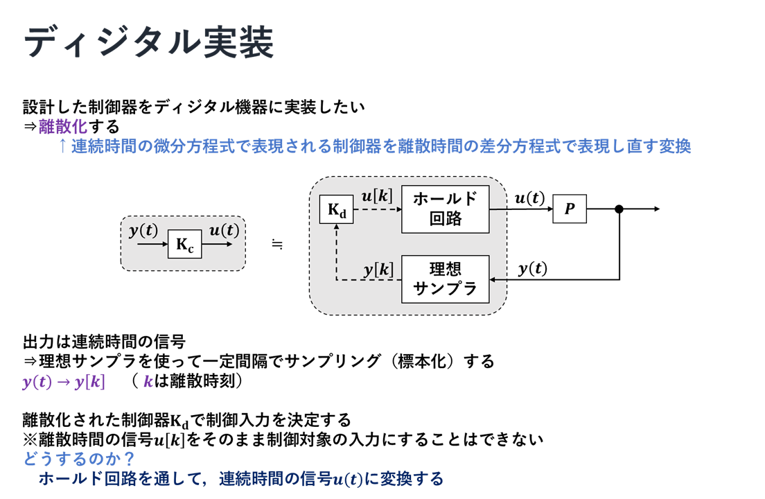
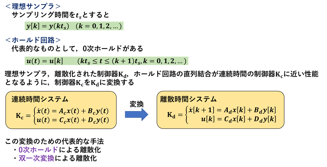
ディジタル実装
以下にディジタル実装についてまとめたものを示す.
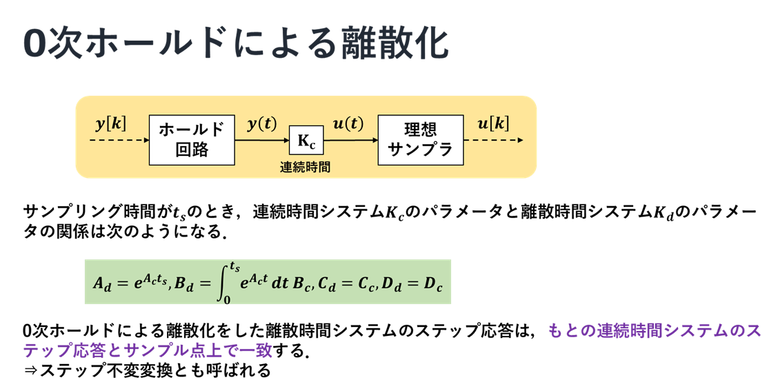
0次ホールドによる離散化
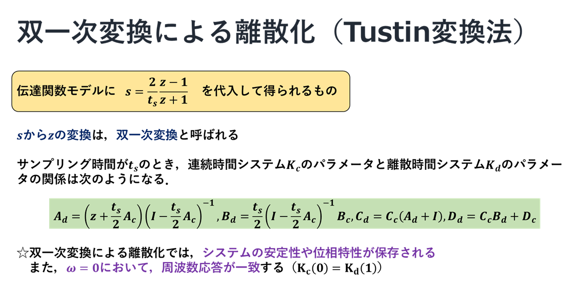
双一次変換による離散化
実装
先ほどの説明に従って,以下にソースコードとそのときの出力を示す.
ソースコード:連続時間システムから離散時間システムへの変換
transform_c2d.py
"""
2021/04/11
@Yuya Shimizu

連続時間システムから離散時間システムへの変換
"""
import matplotlib.pyplot as plt
import numpy as np
from control import tf, c2d
from control.matlab import step
from for_plot import plot_set

P = tf([0, 1], [0.5, 1])
print(P)

### 数式

ts = 0.2    #サンプリング時間

# 0次ホールドによる離散化
Pd1 = c2d(P, ts, method='zoh')
print('離散時間システム(zoh)', Pd1)
# 双一次変換による離散化
Pd2 = c2d(P, ts, method='tustin')
print('離散時間システム(tustin)', Pd2)


### 図示
fig, ax = plt.subplots(1, 2, figsize = (6, 2.6))

# 連続時間システム
Tc = np.arange(0, 3, 0.01)
y, t = step(P, Tc)
ax[0].plot(t, y, ls = '-.')
ax[1].plot(t, y, ls = '-.')

# 離散時間システム(0次ホールドによる離散化)
T = np.arange(0, 3, ts)
y, t = step(Pd1, T)
ax[0].plot(t, y, ls = ' ', marker = 'o', label = 'zoh')

# 離散時間システム(双一次変換による離散化)
y, t = step(Pd2, T)
ax[1].plot(t, y, ls = ' ', marker = 'o', label = 'tustin')

title = ['0th hold', 'Tustin']
for i in range(2):
    ax[i].set_xlabel('t')
    ax[i].set_ylabel('y')
    ax[i].set_title(title[i])
    ax[i].legend()
fig.tight_layout()
plt.show()
出力
    1
---------
0.5 s + 1

離散時間システム(zoh)
  0.3297
----------
z - 0.6703

dt = 0.2

離散時間システム(tustin)
0.1667 z + 0.1667
-----------------
    z - 0.6667

dt = 0.2
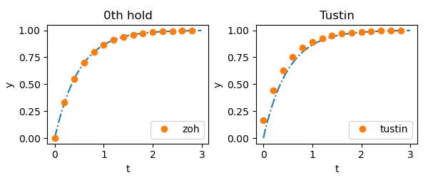
離散化された値がうまく連続時間の信号に乗っていることが確認できる.
ソースコード:連続時間システムから離散時間システムへの変換(時間応答)
入力を$u = 0.5sin(6t) + 0.5cos(8t)$として,離散化方法の差を確認する.
transform_c2d_complex.py
"""
2021/04/11
@Yuya Shimizu

連続時間システムから離散時間システムへの変換(やや複雑)
"""
import matplotlib.pyplot as plt
import numpy as np
from control import tf, c2d
from control.matlab import lsim
from for_plot import plot_set

P = tf([0, 1], [0.5, 1])
print(P)

### 数式

ts = 0.2    #サンプリング時間

# 0次ホールドによる離散化
Pd1 = c2d(P, ts, method='zoh')
print('離散時間システム(zoh)', Pd1)
# 双一次変換による離散化
Pd2 = c2d(P, ts, method='tustin')
print('離散時間システム(tustin)', Pd2)


### 図示
fig, ax = plt.subplots(1, 2, figsize = (6, 2.6))

# 連続時間システム
Tc = np.arange(0, 3, 0.01)
Uc = 0.5 * np.sin(6*Tc) + 0.5*np.cos(8*Tc)
y, t, x0 = lsim(P, Uc, Tc)
ax[0].plot(t, y, ls = '-.')
ax[1].plot(t, y, ls = '-.')

# 離散時間システム(0次ホールドによる離散化)
T = np.arange(0, 3, ts)
U = 0.5 * np.sin(6*T) + 0.5*np.cos(8*T)
y, t, x0 = lsim(Pd1, U, T)
ax[0].plot(t, y, ls = ' ', marker = 'o', label = 'zoh')

# 離散時間システム(双一次変換による離散化)
y, t, x0 = lsim(Pd2, U, T)
ax[1].plot(t, y, ls = ' ', marker = 'o', label = 'tustin')

title = ['0th hold', 'Tustin']
for i in range(2):
    ax[i].set_xlabel('t')
    ax[i].set_ylabel('y')
    ax[i].set_title(title[i])
fig.tight_layout()
fig.suptitle("input; u(t) = 0.5sin(6t) + 0.5cos(8t)")
plt.show()
出力
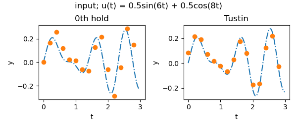
先ほどの入力よりも少し複雑な信号にしたところ,双一次変換のほうが0次ホールドによる離散化よりもうまく離散化できていることが分かる.
ソースコード:ボード線図
周波数応答により,周波数特性を確認する.
transform_c2d_bode.py
"""
2021/04/11
@Yuya Shimizu

ボード線図
"""
import matplotlib.pyplot as plt
import numpy as np
from control import tf, c2d
from control.matlab import bode
from for_plot import plot_set

P = tf([0, 1], [0.5, 1])
print(P)

### 数式

ts = 0.2    #サンプリング時間

# 0次ホールドによる離散化
Pd1 = c2d(P, ts, method='zoh')
print('離散時間システム(zoh)', Pd1)
# 双一次変換による離散化
Pd2 = c2d(P, ts, method='tustin')
print('離散時間システム(tustin)', Pd2)


### 図示
fig, ax = plt.subplots(2, 1)

# 連続時間システム
gain, phase, w = bode(P, np.logspace(-2, 2), Plot = False)
ax[0].semilogx(w, 20*np.log10(gain), ls = '-.', label = 'continuous')
ax[1].semilogx(w, phase*180/np.pi, ls = '-.', label = 'continuous')

# 離散時間システム(0次ホールドによる離散化)
gain, phase, w = bode(Pd1, np.logspace(-2, 2), Plot = False)
ax[0].semilogx(w, 20*np.log10(gain), ls = '-.', label = 'zoh')
ax[1].semilogx(w, phase*180/np.pi, ls = '-.', label = 'zoh')

# 離散時間システム(双一次変換による離散化)
gain, phase, w = bode(Pd2, np.logspace(-2, 2), Plot = False)
ax[0].semilogx(w, 20*np.log10(gain), ls = '-.', label = 'tustin')
ax[1].semilogx(w, phase*180/np.pi, ls = '-.', label = 'tustin')

# 周波数がw=pi/tsのところに線を引く
ax[0].axvline(np.pi/ts, lw = 0.5, c = 'k')
ax[1].axvline(np.pi/ts, lw = 0.5, c = 'k')
ax[1].legend()

ax[0].set_
fig.tight_layout()
plt.show()
出力
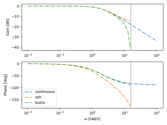
低周波域で連続時間システムとほぼ同じ特徴になっているが,高周波域で特徴が異なっている.0次ホールドによる離散化したシステムのゲイン特性はほぼ連続時間システムのゲイン特性に近くなっているが,位相が大きくずれていることが確認できる.一方,双一次変換で離散化したシステムでは,位相特性が連続時間の位相特性に近くなっているこ確認できる.
感想
ようやく参考書の内容をすべて終えた.最後は,ディジタル実装ということで主に離散化について学んだが,離散化にもいくつかの手法があるのは知らなかった.また,その手法それぞれに特徴があることを学び,用途に合わせて離散化の方法を変えることで望みの実装を実現するのかなと思った.まだまだ経験がないため,いまいちイメージはつかめていないが,それについては経験していく中で学んでいけたらと思う.
参考文献
Pyhtonによる制御工学入門 南 祐樹 著 オーム社