勾配降下法とは

訓練テストに対してコストが最小になるように、モデルパラメータを少しづつ操作し、モデルを訓練テストに対して適合したパラメータに収束させる方法です。
ここではバッチ勾配降下法、確率的勾配降下法、ミニバッチ勾配降下法について触れます。
本記事のコードはHands-on Machine Learning with Scikit-Learn and TensorFlowをもとに作成しました。

線形回帰モデル

今回は線形回帰モデルの訓練を目標にします。

線形回帰モデルは以下のような形になります。

\bar{y}=\theta_0+\theta_1x_1+\cdots+\theta_nx_n

$\bar{y}$：予測された値
n：特徴量数
$x_i$：i番目の特徴量の値
$\theta_j$：j番目のモデルのパラメータ

ベクトル形式で表示すると

\bar{y} = h_\theta(x)=\theta^T\cdot x

$\theta$：モデルのパラメータベクトル
x：特徴量ベクトル ($x_0$=1)

線形回帰モデルを訓練するには、モデルが訓練セットに対して最も適合するパラメータを設定することです。
回帰モデルの一般的な性能指標は二乗平均平方誤差(RMSE)ですが、平均二乗誤差(MSE)を計算する方が簡単です。
つまり線形回帰モデルを訓練するとはMSEの値が最小になるようなモデルパラメータを求めるということになります。

MSE(X, \theta)=\frac{1}{m}\sum_{i=1}^{m}(\theta^T\cdot x^{(i)}-y^{(i)})^2

勾配降下法

勾配降下法はコスト関数を最小にするためにパラメータを繰り返し操作して最適なパラメータを算出します。
パラメータベクトル$\theta$について誤差関数の局所的な勾配を測定し、降下の方向に進めていきます。
勾配が0になればコスト関数を最小にするパラメータを見つけることができたことになります。

今回は$y=4+3x+gausian\ noise$を勾配降下法により学習することを目指します。

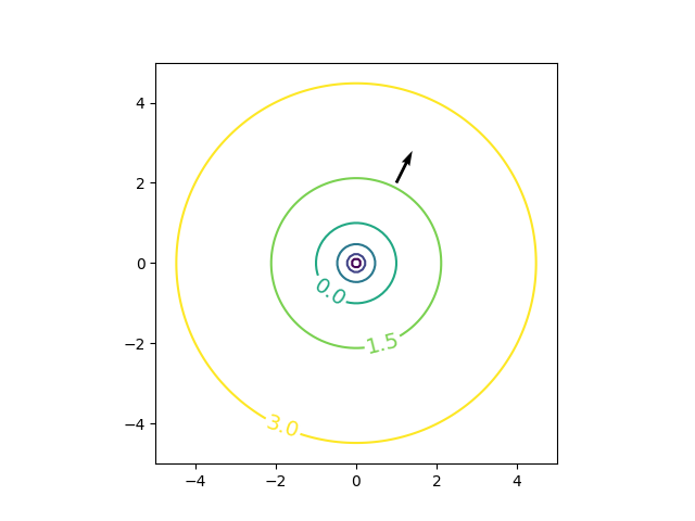
勾配ベクトルについて

高校の美しい物語にて分かりやすく解説してくれています。

$f(x, y) = log(x^2+y^2)$においてx=1, y=2での勾配ベクトルは

\frac{\delta f}{\delta x}=\frac{2x}{x^2+y^2} \\
\frac{\delta f}{\delta y}=\frac{2y}{x^2+y^2}

より、勾配ベクトル$\Delta||f||=(\frac{2}{5}, \frac{4}{5})$となります。

勾配ベクトルの向き：今いる点からちょっと動いたときに関数の値が一番大きくなる向き
勾配ベクトルの大きさは：（Cが小さいもとで）その向きにC進むと関数値は$C||\Delta f||$くらい増えるか

gradient vector	plot 3d

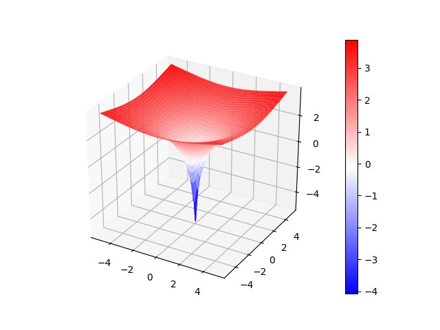つまり、勾配ベクトルの逆向きに進めば最小コストになるパラメータにたどり着くことができそうというイメージがつかめればOKです。

バッチ勾配降下法

線形回帰モデルにおいて最適なパラメータはコスト関数であるMSEを最小にすることのできるパラメータでした。
MSEの勾配ベクトルに注目すれば最適なパラメータを見つけることができそうです。

MSE(X, \theta)=\frac{1}{m}\sum_{i=1}^{m}(\theta^T\cdot x^{(i)}-y^{(i)})^2

パラメータ$\theta_i$についてのコスト関数の偏微分$\frac{\partial}{\partial\theta_j}MSE(\theta)$は以下のようになります。

\frac{\partial}{\partial\theta_j}MSE(\theta)=\frac{2}{m}\sum_{i=1}^{m}(\theta^T \cdot x^{(i)}-y^{(i)})x_j^{(i)}

関数の勾配ベクトルは

\nabla_\theta MSE(\theta)=
\left(
\begin{matrix}
\frac{\partial}{\partial\theta_0}MSE(\theta) \\
\frac{\partial}{\partial\theta_1}MSE(\theta) \\
\vdots \\
\frac{\partial}{\partial\theta_n}MSE(\theta) 
\end{matrix}
\right)
= \frac{2}{m}X^T\cdot (X\cdot \theta - y)

勾配ベクトルの逆の方向に向かえば下に向かうので、$\theta$から$\nabla_\theta MSE(\theta)$を引くことによりパラメータを更新していきます。

\theta^{next\ step}=\theta-\eta\nabla_\theta MSE(\theta)

$\eta$は学習率といい、どの程度勾配を下るかを決めます。
学習率がどのような影響を与えるか実装して確認してみます。

gradient_descent/batch_gradient.py

#coding:utf-8
import numpy as np
import matplotlib.pyplot as plt

np.random.seed(42)

eta = 0.1 # 学習率
n_iterations = 100 # エポック数
m = 100 # データ数

X = 2 * np.random.rand(m, 1)
y = 4 + 3 * X + np.random.randn(m, 1)
X_b = np.c_[np.ones((m, 1)), X]  # add x0 = 1 to each instance

theta = np.random.randn(2, 1)

plt.plot(X, y, "ob")

for iterations in range(n_iterations):
    gradients = 2/float(m) * X_b.T.dot(X_b.dot(theta) - y)
    theta = theta - eta * gradients

    X_new = np.array([[0], [2]])
    X_new_b = np.c_[np.ones((2, 1)), X_new]
    y_predict = X_new_b.dot(theta)

    if(iterations<10):
        plt.plot(X_new, y_predict, "b-")
    elif(iterations==n_iterations-1):
        plt.plot(X_new, y_predict, "r-")

plt.xlabel("x")
plt.ylabel("y")
plt.title(r"$\eta={}$".format(eta), fontsize=16)
plt.axis([0, 2, 0, 15])
plt.savefig("batch_gradient")
plt.show()

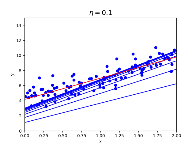
$\eta=0.01$	$\eta=0.1$	$\eta=0.5$

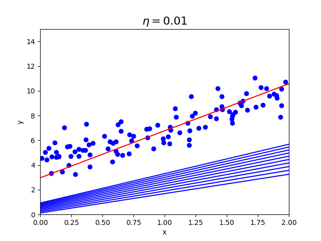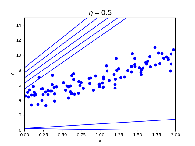学習率が0.01の時より、0.1の方が早く収束していることがわかります。
0.5の時は収束せず、発散してしまっており画像内に収まっていません。
学習率が重要ということがわかると思います。

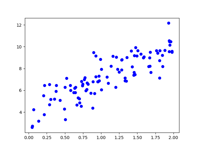
確率的勾配降下法

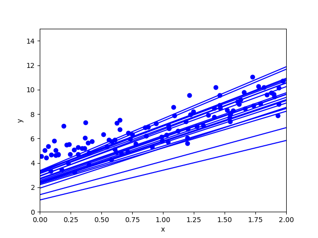
バッチ勾配降下法は勾配を求めるために各ステップで訓練セットをすべて利用しています。そのため訓練セットが多くなればなるほど計算量が増えてしまいます。確率的勾配降下法（Stochastic Gradient Descent）は、各ステップで訓練セットからランダムに一つのインスタンスのみを利用して勾配を計算します。
確率的であるため、バッチ勾配降下法よりも不規則に降下していく特徴があります。

gradient_descent/stochastic_gradient_descent.py

#coding:utf-8

import numpy as np
import matplotlib.pyplot as plt

np.random.seed(42)

n_epochs = 50 # エポック数
m = 100 # データ数

t0, t1 = 5, 50
def learning_schedule(t):
    return t0/float(t+t1)

X = 2 * np.random.rand(m, 1)
y = 4 + 3 * X + np.random.randn(m, 1)
X_b = np.c_[np.ones((m, 1)), X]  # add x0 = 1 to each instance

theta = np.random.randn(2, 1)

plt.plot(X, y, "ob")

for epoch in range(n_epochs):
    for i in range(m):
        random_index = np.random.randint(m)
        xi = X_b[random_index:random_index+1]
        yi = y[random_index:random_index+1]
        gradients = 2.0 * xi.T.dot(xi.dot(theta) - yi)
        eta = learning_schedule(epoch*m + i)
        theta = theta - eta * gradients

        if(epoch==0 and i<20):
            X_new = np.array([[0], [2]])
            X_new_b = np.c_[np.ones((2, 1)), X_new]
            y_predict = X_new_b.dot(theta)
            plt.plot(X_new, y_predict, "b-")

plt.xlabel("x")
plt.ylabel("y")
plt.axis([0, 2, 0, 15])
plt.savefig("stochastic_gradient_descent")
plt.show()

ミニバッチ勾配降下法

各ステップで訓練セットからランダムに選んだ複数のインスタンスを利用して勾配を計算します。

#coding:utf-8

import numpy as np
import matplotlib.pyplot as plt

np.random.seed(42)

m = 100
n_epochs = 50 # エポック数
batch_size = 20 # バッチサイズ

t0, t1 = 200, 1000
def learning_schedule(t):
    return t0/float(t+t1)

X = 2 * np.random.rand(m, 1)
y = 4 + 3 * X + np.random.randn(m, 1)
X_b = np.c_[np.ones((m, 1)), X]  # add x0 = 1 to each instance

theta = np.random.randn(2, 1)

plt.plot(X, y, "ob")

t = 0
for epoch in range(n_epochs):
    shuffled_indices = np.random.permutation(m)
    X_b_shuffled = X_b[shuffled_indices]
    y_shuffled = y[shuffled_indices]
    for i in range(0, m, batch_size):
        t += 1
        xi = X_b_shuffled[i:i+batch_size]
        yi = y_shuffled[i:i+batch_size]
        gradients = 2.0/batch_size*xi.T.dot(xi.dot(theta) - yi)
        eta = learning_schedule(t)
        theta = theta - eta*gradients

        if(i<20):
            X_new = np.array([[0], [2]])
            X_new_b = np.c_[np.ones((2, 1)), X_new]
            y_predict = X_new_b.dot(theta)
            plt.plot(X_new, y_predict, "b-")

plt.xlabel("x")
plt.ylabel("y")
plt.axis([0, 2, 0, 15])
plt.savefig("minibatch_gradient_descent")
plt.show()

確率的勾配降下法	ミニバッチ勾配降下法

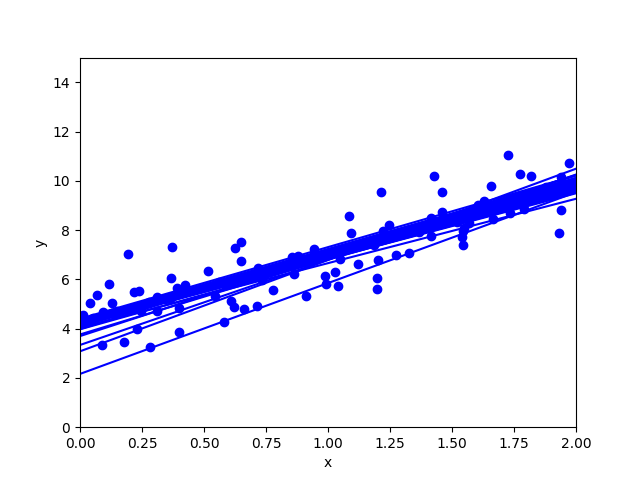ミニバッチ勾配降下法が早く収束していることがわかります。

参照

Hands-on Machine Learning with Scikit-Learn and TensorFlow
確率的勾配降下法とは何か、をPythonで動かして解説する