はじめに
スペクトログラムという音分析手法を使うと,為替データを画像として扱えます.これはCNNと相性がいいかもしれない??と思いまして,スペクトログラムを入力データとするAIで為替予測ができないか検討してみました.
スペクトログラムとは
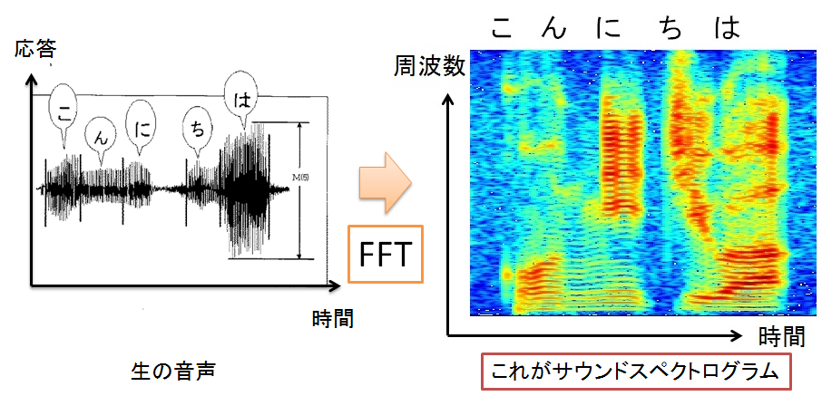
図1 サウンドスペクトログラム
出所:http://blog.media.teu.ac.jp/2015/05/post-0ec1.html
スペクトログラムは時系列波形を3次元グラフ(時間,周波数,波の強さ)で表現したものです.例えば,”こんにちは”をスペクトログラムにすると図1の様になります.
1分足からスペクトログラムを作る
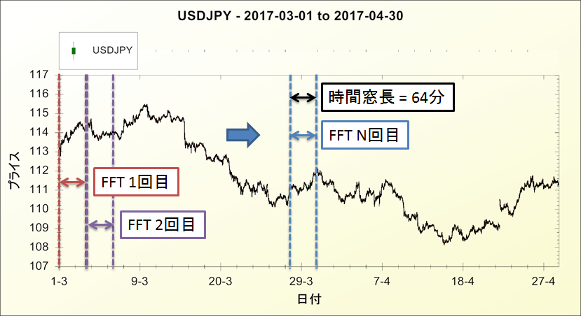
図2 USD/JPY1分足(2017/3/1~2017/4/30)
1分足とは四本値(始値,高値,安値,終値)と出来高を1分ごとに記録したデータです.図2の1分足を例にスペクトログラムの作り方を説明します.
まずは1分足を64分ごとに切り取って何回もFFTします.切り取る幅(時間窓長)はオーバーラップしません.
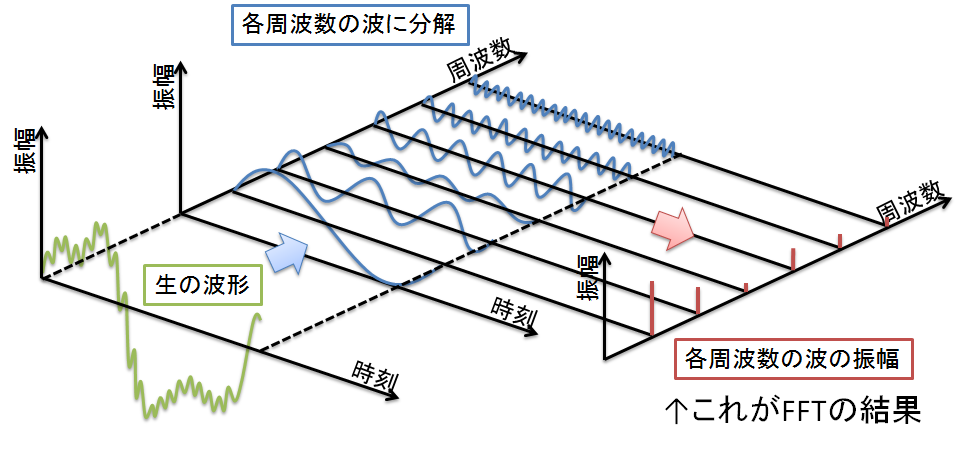
図3 FFTの概要
FFTとは複雑な波を周波数が異なる複数のsin波の重ね合わせとして表現することです.FFTの結果からどの周波数の波の影響が大きいか知ることができます.
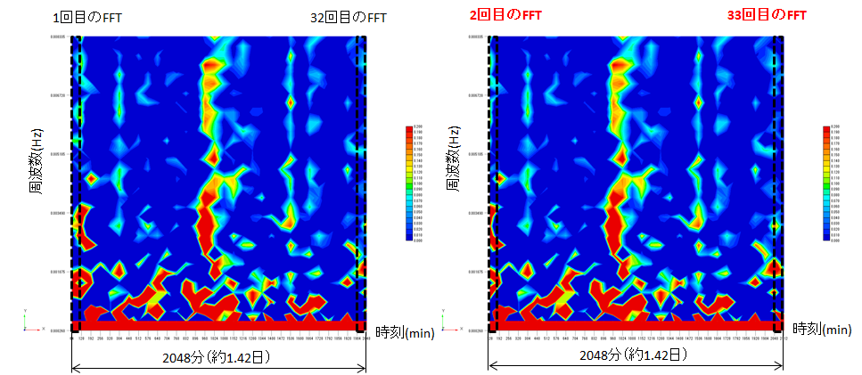
図4 終値のFFT(実部)から作ったスペクトログラム
FFTの結果を左から順番に,1回目,2回目,3回目,,,32回目と並べて行くと,図4の様なスペクトログラムが作成できます.この図のコンターは各時刻,各周波数における波の強さを表しています.続いて,2~33回目のFFTでスペクトログラムを作る,3~34回目のFFTでスペクトログラムを作る,,,と繰り返して行けばたくさんのスペクトログラムが作れるという訳です.
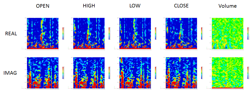
図5 四本値と出来高のFFT(実部,虚部)から作ったスペクトログラム
さらに始値,高値,安値,終値,出来高について,実部と虚部のスペクトログラムを作成します.これら10枚のスペクトログラムとスペクトログラムの最終時刻の1分後の終値が上がるか,下がるかを記録したラベルが1つのデータセットになります.
※FFTの結果は複素数です.そのため,実部と虚部に対してスペクトログラムが作成できます.
AIに学習させる
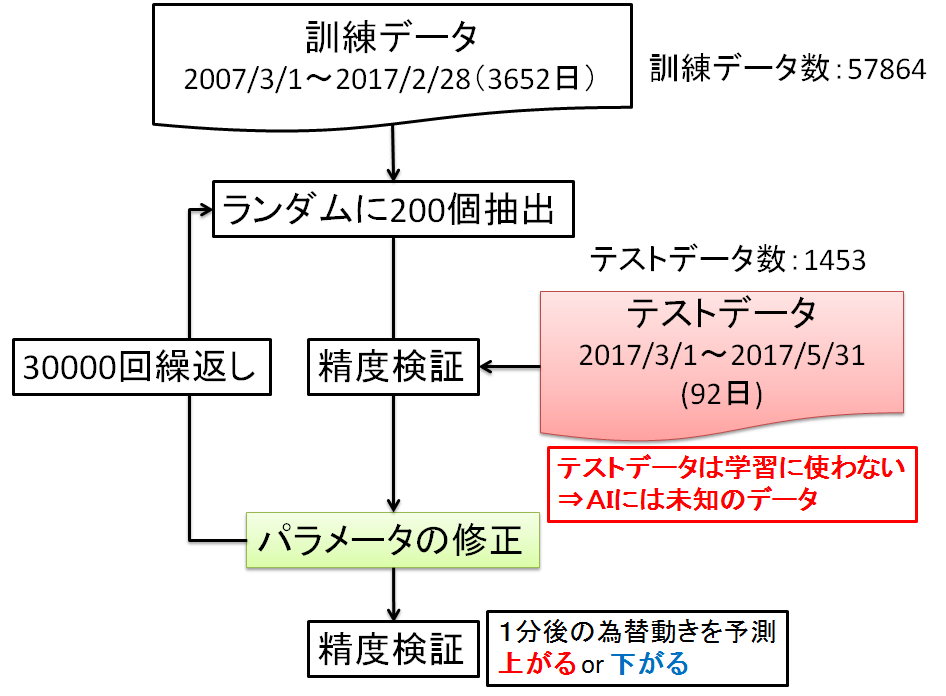
図6 学習フロー
AIには訓練データ(10年)のみを学習させます.そしてテストデータ(3か月)に対して正解率を求めます.CNNは下記の構造にしました.DeepLearningの仕組みに関しては説明を割愛させて頂きます.分析に用いたコードはAppendixをご覧下さい.
input ‐ conv ‐ relu ‐ conv ‐ relu ‐ pool ‐
conv ‐ relu ‐ conv ‐ relu ‐ pool ‐
conv ‐ relu ‐ conv ‐ relu ‐ pool ‐
conv ‐ relu ‐ conv ‐ relu ‐ pool ‐
affine ‐ relu ‐ affine ‐ softmax ‐ output
結果
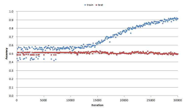
図7 精度検証結果
テストデータに対する正解率は上がりませんでした...残念です!
終わりに
今回作成したスペクトログラムを見ると,低い周波数に強い応答があります.スペクトログラムの周波数レンジを小さくした方が良いかもしれません.周波数レンジを小さくする方法として以下の2つがあります.
1.為替データのサンプリング周波数を小さくする.(15分足や30分足を使う.)
為替データのサンプリング周波数がfsの時,FFT結果の最大周波数はfs/2になります.よってサンプリング周波数を小さくするとスペクトログラムの周波数レンジを小さくできます.ただし,為替データの粒度は粗くなります.
2.FFTのサンプリング点数を増やす.(時間窓長を長くする.)
サンプリング点数がN点のFFTでは,N/2個の波に分解することができます.1で述べた様に,FFT結果の最大周波数はfs/2になりますので,FFT結果の最小周波数はfs/Nになります.よってサンプリング点数を増やすことで,より低い周波数について細かく分析することが可能です.ただし,スペクトログラムのサイズが大きくなるので,計算コストが増加します.
Yu-Nie
Appendix
分析対象とした為替データは以下からダウンロードできます.
USDJPY_20070301_20170228_1min.csv
USDJPY_20170301_20170531_1min.csv
以下は分析に使ったコードです.
# -*- coding: utf-8 -*-
"""
Created on Mon Oct 17 08:54:14 2016
@author: izumiy
The MIT License (MIT)
Copyright (c) 2016 Koki Saitoh
Permission is hereby granted, free of charge, to any person obtaining a copy
of this software and associated documentation files (the "Software"), to deal
in the Software without restriction, including without limitation the rights
to use, copy, modify, merge, publish, distribute, sublicense, and/or sell
copies of the Software, and to permit persons to whom the Software is
furnished to do so, subject to the following conditions:
The above copyright notice and this permission notice shall be included in all
copies or substantial portions of the Software.
THE SOFTWARE IS PROVIDED "AS IS", WITHOUT WARRANTY OF ANY KIND, EXPRESS OR
IMPLIED, INCLUDING BUT NOT LIMITED TO THE WARRANTIES OF MERCHANTABILITY,
FITNESS FOR A PARTICULAR PURPOSE AND NONINFRINGEMENT. IN NO EVENT SHALL THE
AUTHORS OR COPYRIGHT HOLDERS BE LIABLE FOR ANY CLAIM, DAMAGES OR OTHER
LIABILITY, WHETHER IN AN ACTION OF CONTRACT, TORT OR OTHERWISE, ARISING FROM,
OUT OF OR IN CONNECTION WITH THE SOFTWARE OR THE USE OR OTHER DEALINGS IN THE
SOFTWARE.
"""
import numpy as np
import pickle
"""========================================================================="""
"""レイヤを生成するクラス"""
"""========================================================================="""
"""Affineレイヤの順伝播と逆伝播を求めるクラス======================================="""
class Affine:
def __init__(self, W, b):
self.W = W # パラメータ
self.b = b # バイアス
self.x = None # 入力
self.dW = None # パラメータの勾配
self.db = None # バイアスの勾配
self.original_x_shape = None
def forward(self, x):
self.original_x_shape = x.shape # ベクトルに変換する前のxの形状を記録する
x = x.reshape(x.shape[0], -1) # xが3次元以上の場合,ベクトルに変換する.x.shape[0] = データ数
self.x = x
out = np.dot(self.x, self.W) + self.b
return out
def backward(self, dout):
dx = np.dot(dout, self.W.T) # W.TはWの転置
self.dW = np.dot(self.x.T, dout)
self.db = np.sum(dout, axis=0)
dx = dx.reshape(*self.original_x_shape) # 入力データの形状に戻す(テンソル対応)
return dx
"""SoftMaxレイヤの順伝播と逆伝播を求めるクラス====================================="""
class SoftmaxWithLoss:
def __init__(self):
self.loss = None # 1入力当たりの誤差
self.y = None # softmaxの出力
self.t = None # 正解出力のnp配列(ラベル表現(1xデータ数))
def forward(self, x, t):
self.t = t
self.y = softmax_for_matrix(x) # 入力データが複数ある場合, x = (データ数, 要素数)
# self.y = softmax(x) # 入力データが1つの場合, x = (1, 要素数)
self.loss = cross_entropy_error(self.y, self.t)
return self.loss
def backward(self, dout=1):
batch_size = self.t.shape[0]
if self.t.size == self.y.size: # 教師データがone-hot-vectorの場合
dx = (self.y - self.t) / batch_size
else:
dx = self.y.copy()
dx[np.arange(batch_size), self.t] -= 1
dx = dx / batch_size
return dx
"""Reluレイヤの順伝播と逆伝播を求めるクラス===========================================
# x:入力のnp配列,dout:出力層の勾配"""
class Relu:
def __init__(self):
self.mask = None
def forward(self, x):
self.mask = (x <= 0)
out = x.copy() # outにxをコピー
out[self.mask] = 0
return out
def backward(self, dout):
dout[self.mask] = 0
dx = dout
return dx
# test Relu
# x = np.array([[1.0, -0.5],
# [-2.0, 3.0]])
# y = Relu()
# a = y.forward(x)
# print(a)
# [[ 1. 0.]
# [ 0. 3.]]
# b = y.backward(a)
# print(b)
# [[ 1. 0.]
# [ 0. 3.]]
"""Sigmoidレイヤの順伝播と逆伝播を求めるクラス========================================
# x:入力のnp配列,dout:出力層の勾配"""
class Sigmoid:
def __init__(self):
self.out = None # 順伝播の出力
def forward(self, x):
out = 1 / (1 + np.exp(-x))
self.out = out
return out
def backward(self, dout):
dx = dout * (1.0 - self.out) * self.out
return dx
# test Sigmoid
# x = np.array([[1.0, -0.5],
# [-2.0, 3.0]])
# y = Sigmoid()
# a = y.forward(x)
# print(a)
# [[ 0.73105858 0.37754067]
# [ 0.11920292 0.95257413]]
# b = y.backward(x)
# print(b)
# [[ 0.19661193 -0.11750186]
# [-0.20998717 0.13552998]]
"""畳み込み層を生成するクラス===================================================="""
class Convolution:
def __init__(self, W, b, stride=1, pad=0):
self.W = W
self.b = b
self.stride = stride
self.pad = pad
# 中間データ(backward時に使用)
self.x = None
self.col = None
self.col_W = None
# 重み・バイアスパラメータの勾配
self.dW = None
self.db = None
def forward(self, x):
FN, C, FH, FW = self.W.shape # filter_num, input_channel_num, filter_height, filter_width
N, C, H, W = x.shape # input_num, input_channel_num, input_height, input_width
out_h = int(1 + (H + 2*self.pad - FH) / self.stride) # out_h:出力データの高さ, H:入力データの高さ, pad:パディング幅, FH:フィルターの高さ, stride:ストライド,フィルターを適用する位置の間隔
out_w = int(1 + (W + 2*self.pad - FW) / self.stride) # out_hとout_wが整数になるように,pad, FH, strideを指定する
col = im2col(x, FH, FW, self.stride, self.pad)
col_W = self.W.reshape(FN, -1).T
out = np.dot(col, col_W) + self.b
out = out.reshape(N, out_h, out_w, -1).transpose(0, 3, 1, 2)
self.x = x
self.col = col
self.col_W = col_W
return out
def backward(self, dout):
FN, C, FH, FW = self.W.shape
dout = dout.transpose(0, 2, 3, 1).reshape(-1, FN)
self.db = np.sum(dout, axis=0)
self.dW = np.dot(self.col.T, dout)
self.dW = self.dW.transpose(1, 0).reshape(FN, C, FH, FW)
dcol = np.dot(dout, self.col_W.T)
dx = col2im(dcol, self.x.shape, FH, FW, self.stride, self.pad)
return dx
"""プーリング層を生成するクラス===================================================="""
class Pooling:
def __init__(self, pool_h, pool_w, stride=1, pad=0):
self.pool_h = pool_h
self.pool_w = pool_w
self.stride = stride
self.pad = pad
self.x = None
self.arg_max = None
def forward(self, x):
N, C, H, W = x.shape
out_h = int(1 + (H + 2*self.pad - self.pool_h) / self.stride) # out_h:出力データの高さ, H:入力データの高さ, pad:パディング幅, pool_h:フィルターの高さ, stride:ストライド,フィルターを適用する位置の間隔
out_w = int(1 + (W + 2*self.pad - self.pool_w) / self.stride) # out_hとout_wが整数になるように,pad, FH, strideを指定する
col = im2col(x, self.pool_h, self.pool_w, self.stride, self.pad)
col = col.reshape(-1, self.pool_h*self.pool_w)
arg_max = np.argmax(col, axis=1)
out = np.max(col, axis=1)
out = out.reshape(N, out_h, out_w, C).transpose(0, 3, 1, 2)
self.x = x
self.arg_max = arg_max
return out
def backward(self, dout):
dout = dout.transpose(0, 2, 3, 1)
pool_size = self.pool_h * self.pool_w
dmax = np.zeros((dout.size, pool_size))
dmax[np.arange(self.arg_max.size), self.arg_max.flatten()] = dout.flatten()
dmax = dmax.reshape(dout.shape + (pool_size,))
dcol = dmax.reshape(dmax.shape[0] * dmax.shape[1] * dmax.shape[2], -1)
dx = col2im(dcol, self.x.shape, self.pool_h, self.pool_w, self.stride, self.pad)
return dx
"""ドロップアウト層を生成するクラス=================================================="""
class Dropout:
"""
http://arxiv.org/abs/1207.0580
"""
def __init__(self, dropout_ratio=0.5):
self.dropout_ratio = dropout_ratio
self.mask = None
def forward(self, x, train_flg=True):
if train_flg: # 学習
self.mask = np.random.rand(*x.shape) > self.dropout_ratio
return x * self.mask
else: # テスト
return x * (1.0 - self.dropout_ratio)
def backward(self, dout):
return dout * self.mask
"""========================================================================="""
"""画像⇔行列の変換を行う関数"""
"""========================================================================="""
"""画像を行列へ変換する関数===================================================="""
def im2col(input_data, filter_h, filter_w, stride=1, pad=0):
"""
Parameters
----------
input_data : (データ数, チャンネル, 高さ, 幅)の4次元配列からなる入力データ
filter_h : フィルターの高さ
filter_w : フィルターの幅
stride : ストライド
pad : パディング
Returns
-------
col : 2次元配列
"""
N, C, H, W = input_data.shape
out_h = (H + 2*pad - filter_h)//stride + 1
out_w = (W + 2*pad - filter_w)//stride + 1
img = np.pad(input_data, [(0,0), (0,0), (pad, pad), (pad, pad)], 'constant')
col = np.zeros((N, C, filter_h, filter_w, out_h, out_w))
for y in range(filter_h):
y_max = y + stride*out_h
for x in range(filter_w):
x_max = x + stride*out_w
col[:, :, y, x, :, :] = img[:, :, y:y_max:stride, x:x_max:stride]
col = col.transpose(0, 4, 5, 1, 2, 3).reshape(N*out_h*out_w, -1)
return col
"""行列を画像へ変換する関数===================================================="""
def col2im(col, input_shape, filter_h, filter_w, stride=1, pad=0):
"""
Parameters
----------
col :
input_shape : 入力データの形状(例:(10, 1, 28, 28))
filter_h :
filter_w
stride
pad
Returns
-------
"""
N, C, H, W = input_shape
out_h = (H + 2*pad - filter_h)//stride + 1
out_w = (W + 2*pad - filter_w)//stride + 1
col = col.reshape(N, out_h, out_w, C, filter_h, filter_w).transpose(0, 3, 4, 5, 1, 2)
img = np.zeros((N, C, H + 2*pad + stride - 1, W + 2*pad + stride - 1))
for y in range(filter_h):
y_max = y + stride*out_h
for x in range(filter_w):
x_max = x + stride*out_w
img[:, :, y:y_max:stride, x:x_max:stride] += col[:, :, y, x, :, :]
return img[:, :, pad:H + pad, pad:W + pad]
"""========================================================================="""
"""ファイル入出力を行う関数"""
"""========================================================================="""
"""インプットと正解出力を読み込む関数=============================================="""
def open_input_for_spectrogram(file_name, input_data_col):
input_date_list = input_data_col
input_date_tuple = tuple(input_date_list)
input = np.loadtxt(file_name, delimiter = ",", usecols = input_date_tuple)
return input
def open_label_for_spectrogram(file_name, label_col):
label = np.loadtxt(file_name, delimiter = ",", usecols = label_col, dtype = np.int)
return label
"""========================================================================="""
"""損失関数の値を求める関数"""
"""========================================================================="""
"""二乗和誤差を求める関数======================================================"""
def mean_squared_error(y, t):
return 0.5 * np.sum((y-t)**2)
# test mean_squared_error(y, t)
# t = [0, 0, 1, 0, 0, 0, 0, 0, 0, 0]
# y = [0.1, 0.05, 0.6, 0.0, 0.05, 0.1, 0.0, 0.1, 0.0, 0.0]
# print(mean_squared_error(np.array(y), np.array(t)))
# 0.0975
"""交差エントロピー誤差を求める関数==================================================
# y:ニューラルネットワークのアウトプット np配列(データ数xラベル数)
# t:正解出力のone-hot表現 np配列(データ数xラベル数)"""
def cross_entropy_error_one_hot(y, t):
delta = 1e-7
if y.ndim == 1: # 配列の次元数が1の時
t = t.reshape(1, t.size) # .sizeは配列の要素数を求める
y = y.reshape(1, y.size)
batch_size = y.shape[0] # y.shape[0]は配列yの行数 = yのデータ数
return -np.sum(t * np.log(y + delta)) / batch_size #np.log(0)はマイナス無限大になってしまうため,微小な値deltaを追加してマイナス無限大を発生させないようにする
# test cross_entropy_error_one_hot(y, t)
# t = [0, 0, 1, 0, 0, 0, 0, 0, 0, 0]
# y = [0.1, 0.05, 0.6, 0.0, 0.05, 0.1, 0.0, 0.1, 0.0, 0.0]
# print(cross_entropy_error_one_hot(np.array(y), np.array(t)))
# 0.510825457099
""" 交差エントロピー誤差を求める関数=================================================
# y:ニューラルネットワークのアウトプット np配列(データ数xラベル数)
# t:正解出力のone-hot表現 np配列(1xデータ数)"""
def cross_entropy_error(y, t):
if y.ndim == 1:
t = t.reshape(1, t.size) # .sizeは配列の要素数を求める
y = y.reshape(1, y.size)
batch_size = y.shape[0] # データ数を取得
return -np.sum(np.log(y[np.arange(batch_size), t])) / batch_size
# test cross_entropy_error(y, t)
# t = [2]
# y = [0.1, 0.05, 0.6, 0.0, 0.05, 0.1, 0.0, 0.1, 0.0, 0.0]
# print(cross_entropy_error(np.array(y), np.array(t)))
# 0.510825623766
"""========================================================================="""
"""活性化関数"""
"""========================================================================="""
"""np配列をソフトマックス関数値に変換する関数==========================================
# a:np配列, aはベクトル限定, 2次元配列は非対応"""
def softmax(a):
c = np.max(a) # np配列aの最大要素を取得
exp_a = np.exp(a - c) # オーバーフロー対策
sum_exp_a = np.sum(exp_a)
y = exp_a / sum_exp_a
return y
# test softmax(a)
# a = np.array([0.3, 2.9, 4.0])
# y = softmax(a)
# print(y)
# [ 0.01821127 0.24519181 0.73659691]
# print(np.sum(y))
# 1.0
"""np配列をソフトマックス関数値に変換する関数==========================================
# a:np配列, aは2次元配列"""
def softmax_for_matrix(a):
count = 0
y = np.zeros_like(a)
for a_row in a:
c = np.max(a_row) # np配列aの最大要素を取得
exp_a_row = np.exp(a_row - c) # オーバーフロー対策
sum_exp_a_row = np.sum(exp_a_row)
y[count,:] = exp_a_row / sum_exp_a_row
count += 1
return y
# test softmax(a)
# a = np.array([[0.3, 2.9, 4.0],
# [0.2, 3.0, 4.3],
# [0.3, 2.0, 6.0]])
# y = softmax(a)
# print(y)
# [[ 0.01821127 0.24519181 0.73659691]
# [ 0.01285596 0.21141172 0.77573232]
# [ 0.00327502 0.0179273 0.97879767]]
"""========================================================================="""
"""数値微分によって勾配を求める関数"""
"""========================================================================="""
"""多層のニューラルネットワークのパラメータの勾配を求める関数,数値微分=======================
# net:多層のニューラルネットワーククラス, params_W:勾配を求めるパラメータ, rows_W:パラメータの行数
# columns_W:パラメータの列数, x:入力, t:正解出力(ラベル表現)"""
def numerical_gradient_for_multi_net_W(net, params_W, rows_W, columns_W, x, t):
h = 1e-4 # 0.0001
grad_W = np.zeros_like(params_W) # params_Wと同じ形状の配列を生成
for row in range(0, rows_W):
for column in range(0, columns_W):
tmp_val = params_W[row, column]
# f(x+h)の計算
params_W[row, column] = tmp_val + h
fxh1 = net.loss(x, t) # 交差エントロピー誤差
# f(x-h)の計算
params_W[row, column] = tmp_val - h
fxh2 = net.loss(x, t) # 交差エントロピー誤差
grad_W[row, column] = (fxh1 - fxh2) / (2*h)
params_W[row, column] = tmp_val
return grad_W
"""多層のニューラルネットワークのバイアスの勾配を求める関数,数値微分========================
# net:多層のニューラルネットワーククラス, params_b:勾配を求めるバイアス,
# columns_b:バイアスの列数, x:入力, t:正解出力(ラベル表現)"""
def numerical_gradient_for_multi_net_b(net, params_b, columns_b, x, t):
h = 1e-4 # 0.0001
grad_b = np.zeros_like(params_b) # net.Wと同じ形状の配列を生成
for column in range(0, columns_b):
tmp_val = params_b[column]
# f(x+h)の計算
params_b[column] = tmp_val + h
fxh1 = net.loss(x, t)
# f(x-h)の計算
params_b[column] = tmp_val - h
fxh2 = net.loss(x, t)
grad_b[column] = (fxh1 - fxh2) / (2*h)
params_b[column] = tmp_val
return grad_b
# test numerical_gradient and backprop_gradient
# network = TwoLayerNet(input_size = 7, hidden_size = 14, output_size = 2)
# input = np.array([])
# label = np.array([])
# input = open_input()
# label = open_label()
# grad_numerical = network.numerical_gradient_for_multi_net(input, label)
# grad_backprop = network.gradient(input, label)
# print(grad_numerical)
# print(grad_backprop)
# for key in grad_numerical.keys():
# diff = np.average(np.abs(grad_backprop[key] - grad_numerical[key]))
# print(key + ":" + str(diff))
# b1:7.34990135764e-08
# b2:1.44404453672e-11
# W1:5.60468518899e-05
# W2:9.17962625938e-12
"""========================================================================="""
"""パラメータの更新方法"""
"""========================================================================="""
"""SGD"""
class SGD:
def __init__(self, lr=0.0005):
self.lr = lr
def update(self, params, grads):
for key in params.keys():
params[key] -= self.lr * grads[key]
"""Momentum"""
class Momentum:
def __init__(self, lr=0.0005, momentum=0.9):
self.lr = lr
self.momentum = momentum
self.v = None
def update(self, params, grads):
if self.v is None:
self.v = {}
for key, val in params.items():
self.v[key] = np.zeros_like(val)
for key in params.keys():
self.v[key] = self.momentum * self.v[key] - self.lr * grads[key]
params[key] += self.v[key]
"""AdaGrad"""
class AdaGrad:
def __init__(self, lr=0.0005):
self.lr = lr
self.h = None
def update(self, params, grads):
if self.h is None:
self.h = {}
for key, val in params.items():
self.h[key] = np.zeros_like(val)
for key in params.keys():
self.h[key] += grads[key] * grads[key]
params[key] -= self.lr * grads[key] / (np.sqrt(self.h[key]) + 1e-7)
"""Nesterov's Accelerated Gradient (http://arxiv.org/abs/1212.0901)"""
class Nesterov:
def __init__(self, lr=0.01, momentum=0.9):
self.lr = lr
self.momentum = momentum
self.v = None
def update(self, params, grads):
if self.v is None:
self.v = {}
for key, val in params.items():
self.v[key] = np.zeros_like(val)
for key in params.keys():
self.v[key] *= self.momentum
self.v[key] -= self.lr * grads[key]
params[key] += self.momentum * self.momentum * self.v[key]
params[key] -= (1 + self.momentum) * self.lr * grads[key]
"""RMSprop"""
class RMSprop:
def __init__(self, lr=0.01, decay_rate = 0.99):
self.lr = lr
self.decay_rate = decay_rate
self.h = None
def update(self, params, grads):
if self.h is None:
self.h = {}
for key, val in params.items():
self.h[key] = np.zeros_like(val)
for key in params.keys():
self.h[key] *= self.decay_rate
self.h[key] += (1 - self.decay_rate) * grads[key] * grads[key]
params[key] -= self.lr * grads[key] / (np.sqrt(self.h[key]) + 1e-7)
"""Adam (http://arxiv.org/abs/1412.6980v8)"""
class Adam:
def __init__(self, lr=0.001, beta1=0.9, beta2=0.999):
self.lr = lr
self.beta1 = beta1
self.beta2 = beta2
self.iter = 0
self.m = None
self.v = None
def update(self, params, grads):
if self.m is None:
self.m, self.v = {}, {}
for key, val in params.items():
self.m[key] = np.zeros_like(val)
self.v[key] = np.zeros_like(val)
self.iter += 1
lr_t = self.lr * np.sqrt(1.0 - self.beta2**self.iter) / (1.0 - self.beta1**self.iter)
for key in params.keys():
#self.m[key] = self.beta1*self.m[key] + (1-self.beta1)*grads[key]
#self.v[key] = self.beta2*self.v[key] + (1-self.beta2)*(grads[key]**2)
self.m[key] += (1 - self.beta1) * (grads[key] - self.m[key])
self.v[key] += (1 - self.beta2) * (grads[key]**2 - self.v[key])
params[key] -= lr_t * self.m[key] / (np.sqrt(self.v[key]) + 1e-7)
#unbias_m += (1 - self.beta1) * (grads[key] - self.m[key]) # correct bias
#unbisa_b += (1 - self.beta2) * (grads[key]*grads[key] - self.v[key]) # correct bias
#params[key] += self.lr * unbias_m / (np.sqrt(unbisa_b) + 1e-7)
"""========================================================================="""
"""為替を予測するAI"""
"""========================================================================="""
"""ディープレイヤのCNNを生成するクラス for 為替予測AI ==============================="""
class DeepConvNet_for_exchange:
"""
conv - relu - conv- relu - pool -
conv - relu - conv- relu - pool -
conv - relu - conv- relu - pool -
affine - relu - affine - softmax
"""
def __init__(self, input_dim=(2, 32, 1024),
conv_param_1 = {'filter_num':16, 'filter_size':3, 'pad':1, 'stride':1},
conv_param_2 = {'filter_num':16, 'filter_size':3, 'pad':1, 'stride':1},
conv_param_3 = {'filter_num':32, 'filter_size':3, 'pad':1, 'stride':1},
conv_param_4 = {'filter_num':32, 'filter_size':3, 'pad':1, 'stride':1},
conv_param_5 = {'filter_num':64, 'filter_size':3, 'pad':1, 'stride':1},
conv_param_6 = {'filter_num':64, 'filter_size':3, 'pad':1, 'stride':1},
hidden_size=50, output_size=2):
""" 畳み込み層,プーリング層の出力サイズ
OH = (H + 2P - FH) / S + 1
OW = (W + 2P - FW) / S + 1
OH, OWは整数が整数になるように,P, FH, FW, Sを指定する.
P:パディング幅, FH:フィルター高さ, FW:フィルター幅, S:ストライド
OH:出力画像の高さ, OW:出力画像の幅, H:入力画像の高さ, W:入力画像の幅
"""
# 重みの初期化===========
# 各層のニューロン1つあたりがつながりを持つ前層のニューロンの数
# ex)
# input - Conv1 : 入力のチャンネル数 x Conv1のフィルターサイズ x Conv1のフィルターサイズ
# Conv1 - Conv2 : Conv1のフィルター数 x Conv2のフィルターサイズ x Conv2のフィルターサイズ
# Conv2 - Affine1 : Conv2の要素数 = Conv2_filter_num x Conv2_h x Conv2_w
# Affine1 - Affine2 : Affine1 の hidden_size
# パラメータの初期化===========
pre_node_nums = np.array([input_dim[0]*3*3, 16*3*3, 16*3*3, 32*3*3, 32*3*3, 64*3*3, 64*3*3, hidden_size])
weight_init_scales = np.sqrt(2.0 / pre_node_nums) # ReLUを使う場合に推奨される初期値
height = int(input_dim[1] / 2**3) # 2**num_pool_layer
width = int(input_dim[2] / 2**3)
self.params = {}
pre_channel_num = input_dim[0]
for idx, conv_param in enumerate([conv_param_1, conv_param_2, conv_param_3, conv_param_4, conv_param_5, conv_param_6]):
self.params['W' + str(idx+1)] = weight_init_scales[idx] * np.random.randn(conv_param['filter_num'], pre_channel_num, conv_param['filter_size'], conv_param['filter_size'])
self.params['b' + str(idx+1)] = np.zeros(conv_param['filter_num'])
pre_channel_num = conv_param['filter_num']
self.params['W7'] = weight_init_scales[6] * np.random.randn(64*height*width, hidden_size) # 入力データのフィルターサイズ x 高さ x 幅
self.params['b7'] = np.zeros(hidden_size)
self.params['W8'] = weight_init_scales[7] * np.random.randn(hidden_size, output_size)
self.params['b8'] = np.zeros(output_size)
# レイヤの生成===========
self.layers = []
self.layers.append(Convolution(self.params['W1'], self.params['b1'],
conv_param_1['stride'], conv_param_1['pad']))
self.layers.append(Relu())
self.layers.append(Convolution(self.params['W2'], self.params['b2'],
conv_param_2['stride'], conv_param_2['pad']))
self.layers.append(Relu())
self.layers.append(Pooling(pool_h=2, pool_w=2, stride=2))
self.layers.append(Convolution(self.params['W3'], self.params['b3'],
conv_param_3['stride'], conv_param_3['pad']))
self.layers.append(Relu())
self.layers.append(Convolution(self.params['W4'], self.params['b4'],
conv_param_4['stride'], conv_param_4['pad']))
self.layers.append(Relu())
self.layers.append(Pooling(pool_h=2, pool_w=2, stride=2))
self.layers.append(Convolution(self.params['W5'], self.params['b5'],
conv_param_5['stride'], conv_param_5['pad']))
self.layers.append(Relu())
self.layers.append(Convolution(self.params['W6'], self.params['b6'],
conv_param_6['stride'], conv_param_6['pad']))
self.layers.append(Relu())
self.layers.append(Pooling(pool_h=2, pool_w=2, stride=2))
self.layers.append(Affine(self.params['W7'], self.params['b7']))
self.layers.append(Relu())
# self.layers.append(Dropout(0.5)) # CIFAR-10データセットの場合,Dropoutを使うと学習が進まない
self.layers.append(Affine(self.params['W8'], self.params['b8']))
# self.layers.append(Dropout(0.5))
self.last_layer = SoftmaxWithLoss()
def predict(self, x, train_flg=False):
for layer in self.layers:
# print('x_shape : ' + str(x.shape))
if isinstance(layer, Dropout):
x = layer.forward(x, train_flg)
else:
x = layer.forward(x)
return x
def loss(self, x, t):
y = self.predict(x, train_flg=True)
return self.last_layer.forward(y, t)
def accuracy(self, x, t):
y = self.predict(x, train_flg=False)
y = np.argmax(y, axis=1)
if t.ndim != 1 : t = np.argmax(t, axis=1)
accuracy = np.sum(y == t) / float(x.shape[0])
return accuracy
def gradient(self, x, t):
# forward
self.loss(x, t)
# backward
dout = 1
dout = self.last_layer.backward(dout)
tmp_layers = self.layers.copy()
tmp_layers.reverse()
for layer in tmp_layers:
dout = layer.backward(dout)
# 設定
grads = {}
for i, layer_idx in enumerate((0, 2, 5, 7, 10, 12, 15, 17)):
grads['W' + str(i+1)] = self.layers[layer_idx].dW
grads['b' + str(i+1)] = self.layers[layer_idx].db
return grads
def save_params(self, file_name="params.pkl"):
params = {}
for key, val in self.params.items():
params[key] = val
with open(file_name, 'wb') as f:
pickle.dump(params, f)
def load_params(self, file_name="params.pkl"):
with open(file_name, 'rb') as f:
params = pickle.load(f)
for key, val in params.items():
self.params[key] = val
for i, layer_idx in enumerate((0, 2, 5, 7, 10, 12, 15, 17)):
self.layers[layer_idx].W = self.params['W' + str(i+1)]
self.layers[layer_idx].b = self.params['b' + str(i+1)]
"""ディープレイヤのCNNを生成するクラス for 為替予測AI ==============================="""
class SuperDeepConvNet_for_exchange:
"""
conv - relu - conv - relu - pool -
conv - relu - conv - relu - pool -
conv - relu - conv - relu - pool -
conv - relu - conv - relu - pool -
affine - relu - affine - softmax
"""
def __init__(self, input_dim=(2, 32, 1024), # channel, height, width
conv_param_1 = {'filter_num':16, 'filter_size':3, 'pad':1, 'stride':1},
conv_param_2 = {'filter_num':16, 'filter_size':3, 'pad':1, 'stride':1},
conv_param_3 = {'filter_num':32, 'filter_size':3, 'pad':1, 'stride':1},
conv_param_4 = {'filter_num':32, 'filter_size':3, 'pad':1, 'stride':1},
conv_param_5 = {'filter_num':32, 'filter_size':3, 'pad':1, 'stride':1},
conv_param_6 = {'filter_num':32, 'filter_size':3, 'pad':1, 'stride':1},
conv_param_7 = {'filter_num':64, 'filter_size':3, 'pad':1, 'stride':1},
conv_param_8 = {'filter_num':64, 'filter_size':3, 'pad':1, 'stride':1},
hidden_size=50, output_size=2):
""" 畳み込み層,プーリング層の出力サイズ
OH = (H + 2P - FH) / S + 1
OW = (W + 2P - FW) / S + 1
OH, OWは整数が整数になるように,P, FH, FW, Sを指定する.
P:パディング幅, FH:フィルター高さ, FW:フィルター幅, S:ストライド
OH:出力画像の高さ, OW:出力画像の幅, H:入力画像の高さ, W:入力画像の幅
"""
# 重みの初期化===========
# 各層のニューロン1つあたりがつながりを持つ前層のニューロンの数
# ex)
# input - Conv1 : 入力のチャンネル数 x Conv1のフィルターサイズ x Conv1のフィルターサイズ
# Conv1 - Conv2 : Conv1のフィルター数 x Conv2のフィルターサイズ x Conv2のフィルターサイズ
# Conv2 - Affine1 : Conv2の要素数 = Conv2_filter_num x Conv2_h x Conv2_w
# Affine1 - Affine2 : Affine1 の hidden_size
pre_node_nums = np.array([input_dim[0]*3*3, 16*3*3, 16*3*3, 32*3*3, 32*3*3, 32*3*3, 32*3*3, 64*3*3, 64*3*3, hidden_size])
weight_init_scales = np.sqrt(2.0 / pre_node_nums) # ReLUを使う場合に推奨される初期値
height = int(input_dim[1] / 2**4) # 2**num_pool_layer
width = int(input_dim[2] / 2**4)
self.params = {}
pre_channel_num = input_dim[0]
for idx, conv_param in enumerate([conv_param_1, conv_param_2, conv_param_3, conv_param_4, conv_param_5, conv_param_6, conv_param_7, conv_param_8]):
self.params['W' + str(idx+1)] = weight_init_scales[idx] * np.random.randn(conv_param['filter_num'], pre_channel_num, conv_param['filter_size'], conv_param['filter_size'])
self.params['b' + str(idx+1)] = np.zeros(conv_param['filter_num'])
pre_channel_num = conv_param['filter_num']
self.params['W9'] = weight_init_scales[8] * np.random.randn(64*height*width, hidden_size) # 入力データのフィルターサイズ x 高さ x 幅
self.params['b9'] = np.zeros(hidden_size)
self.params['W10'] = weight_init_scales[9] * np.random.randn(hidden_size, output_size)
self.params['b10'] = np.zeros(output_size)
# レイヤの生成===========
self.layers = []
self.layers.append(Convolution(self.params['W1'], self.params['b1'],
conv_param_1['stride'], conv_param_1['pad']))
self.layers.append(Relu())
self.layers.append(Convolution(self.params['W2'], self.params['b2'],
conv_param_2['stride'], conv_param_2['pad']))
self.layers.append(Relu())
self.layers.append(Pooling(pool_h=2, pool_w=2, stride=2))
self.layers.append(Convolution(self.params['W3'], self.params['b3'],
conv_param_3['stride'], conv_param_3['pad']))
self.layers.append(Relu())
self.layers.append(Convolution(self.params['W4'], self.params['b4'],
conv_param_4['stride'], conv_param_4['pad']))
self.layers.append(Relu())
self.layers.append(Pooling(pool_h=2, pool_w=2, stride=2))
self.layers.append(Convolution(self.params['W5'], self.params['b5'],
conv_param_5['stride'], conv_param_5['pad']))
self.layers.append(Relu())
self.layers.append(Convolution(self.params['W6'], self.params['b6'],
conv_param_6['stride'], conv_param_6['pad']))
self.layers.append(Relu())
self.layers.append(Pooling(pool_h=2, pool_w=2, stride=2))
self.layers.append(Convolution(self.params['W7'], self.params['b7'],
conv_param_7['stride'], conv_param_7['pad']))
self.layers.append(Relu())
self.layers.append(Convolution(self.params['W8'], self.params['b8'],
conv_param_8['stride'], conv_param_8['pad']))
self.layers.append(Relu())
self.layers.append(Pooling(pool_h=2, pool_w=2, stride=2))
self.layers.append(Affine(self.params['W9'], self.params['b9']))
self.layers.append(Relu())
# self.layers.append(Dropout(0.5)) # CIFAR-10データセットの場合,Dropoutを使うと学習が進まない
self.layers.append(Affine(self.params['W10'], self.params['b10']))
# self.layers.append(Dropout(0.5))
self.last_layer = SoftmaxWithLoss()
def predict(self, x, train_flg=False):
for layer in self.layers:
# print('x_shape : ' + str(x.shape))
if isinstance(layer, Dropout):
x = layer.forward(x, train_flg)
else:
x = layer.forward(x)
return x
def loss(self, x, t):
y = self.predict(x, train_flg=True)
return self.last_layer.forward(y, t)
def accuracy(self, x, t):
y = self.predict(x, train_flg=False)
y = np.argmax(y, axis=1)
if t.ndim != 1 : t = np.argmax(t, axis=1)
accuracy = np.sum(y == t) / float(x.shape[0])
return accuracy
def gradient(self, x, t):
# forward
self.loss(x, t)
# backward
dout = 1
dout = self.last_layer.backward(dout)
tmp_layers = self.layers.copy()
tmp_layers.reverse()
for layer in tmp_layers:
dout = layer.backward(dout)
# 設定
grads = {}
for i, layer_idx in enumerate((0, 2, 5, 7, 10, 12, 15, 17, 20, 22)):
grads['W' + str(i+1)] = self.layers[layer_idx].dW
grads['b' + str(i+1)] = self.layers[layer_idx].db
return grads
def save_params(self, file_name="params.pkl"):
params = {}
for key, val in self.params.items():
params[key] = val
with open(file_name, 'wb') as f:
pickle.dump(params, f)
def load_params(self, file_name="params.pkl"):
with open(file_name, 'rb') as f:
params = pickle.load(f)
for key, val in params.items():
self.params[key] = val
for i, layer_idx in enumerate((0, 2, 5, 7, 10, 12, 15, 17, 20, 22)):
self.layers[layer_idx].W = self.params['W' + str(i+1)]
self.layers[layer_idx].b = self.params['b' + str(i+1)]
"""========================================================================="""
"""DeepConvNetにて為替データを学習する関数"""
"""========================================================================="""
"""為替の時系列データをFFTする関数==============================================="""
"""
・為替の時系列データに対してFFTを連続実行する(実数部と虚数部を出力)
・FFTに使ったデータの直後の為替レートの増減をラベル化する
下がる:0, 上がる:1, 変化無し:2
・上記を連続実行し,1つのnumpy配列にまとめる
"""
def FFT_complex_10(file_name, num_sample, time_start = 0, over_lap = 1, predict_time_inc = 1):
"""始値,高値,安値,終値,Volumeを使用"""
# num_sample:時間窓長に含まれるサンプリング点数(2の乗数にすること)
freq_lines = int(num_sample / 2) # 分析ライン数 = サンプル数 / 2 https://www.onosokki.co.jp/HP-WK/c_support/faq/fft_common/fft_analys_4.htm
spectrogram_idx = 10 * freq_lines + 1 # 2(実数,虚数) x 5(始値,高値,安値,終値,Volume) = 10, 末尾の"+1"はラベル
# print(freq_lines_idx)
"""為替時系列データの読込み"""
print("reading the input file...")
time_series = np.loadtxt(file_name, delimiter = ",", usecols = (2,3,4,5,6), skiprows = 1) # 始値,高値,安値,終値,Volumeをnumpy配列として取得する
num_series_data = time_series.shape[0] # データ数の取得
print("reading the input file is done")
print("num_series_data")
print(num_series_data)
time_end = int(time_start + num_sample)
time_inc = int(num_sample / over_lap) # FFT開始時刻の増分
spectrogram = np.empty((0, spectrogram_idx))
while(time_end < (num_series_data - predict_time_inc)):
print("time_start:" + str(time_start))
"""FFTの実行"""
time_window = time_series[time_start:time_end, :] # 時間窓長だけデータを抽出する
"""2次元配列に対してFFTを行う場合は,分析方向の指定が必要"""
FFT = np.fft.fft(time_window, axis=0) # FFTの実行,結果は複素数として出力される
FFT = FFT[0:freq_lines, :] # ナイキスト周波数以上のデータは削除する
# FFT = np.abs(FFT) # FFTの結果は複素数なので,絶対値にする
FFT_real = np.real(FFT) # FFTの実数部
FFT_imag = np.imag(FFT) # FFTの虚数部
"""ラベル作成"""
# 始値を使用する場合
current_rate = time_series[time_end, 3] # FFTの最終時刻の終値
future = time_end + predict_time_inc # FFTの最終時刻の直後
future_rate = time_series[future, 3] # FFTの最終時刻の直後の終値
if current_rate >= future_rate:
FFT_label = 0
# elif current_rate == future_rate:
# FFT_label = 2
else:
FFT_label = 1
"""FFT結果の結合"""
FFT_complex = np.append(FFT_real, FFT_imag, axis=0)
FFT_complex = FFT_complex.T
print("FFT_complex_shape:" + str(FFT_complex.shape))
FFT_complex = FFT_complex.reshape(-1, 1) # 縦ベクトルに変換する
print("FFT_complex_shape_1d:" + str(FFT_complex.shape))
FFT_complex = np.append(FFT_complex, FFT_label) # ラベルの追記
print("FFT_complex_shape_label_add:" + str(FFT_complex.shape))
FFT_complex = FFT_complex.reshape(1, -1) # 横ベクトルに変換する
print("FFT_complex_shape_label_add_transverse:" + str(FFT_complex.shape))
spectrogram = np.append(spectrogram, FFT_complex, axis=0) # FFTの結果を追記する
print("spectrogram_shape:" + str(spectrogram.shape))
time_start = time_start + time_inc # FFTの開始時刻の更新
time_end = int(time_start + num_sample)
print("num_series_data")
print(num_series_data)
return spectrogram
def FFT_complex_8(file_name, num_sample, time_start = 0, over_lap = 1, predict_time_inc = 1):
"""始値,高値,安値,終値を使用"""
# num_sample:時間窓長に含まれるサンプリング点数(2の乗数にすること)
freq_lines = int(num_sample / 2) # 分析ライン数 = サンプル数 / 2 https://www.onosokki.co.jp/HP-WK/c_support/faq/fft_common/fft_analys_4.htm
spectrogram_idx = 8 * freq_lines + 1 # 2(実数,虚数) x 4(始値,高値,安値,終値) = 8, 末尾の"+1"はラベル
# print(freq_lines_idx)
"""為替時系列データの読込み"""
print("reading the input file...")
time_series = np.loadtxt(file_name, delimiter = ",", usecols = (2,3,4,5), skiprows = 1) # 始値,高値,安値,終値をnumpy配列として取得する
num_series_data = time_series.shape[0] # データ数の取得
print("reading the input file is done")
print("num_series_data")
print(num_series_data)
time_end = int(time_start + num_sample)
time_inc = int(num_sample / over_lap) # FFT開始時刻の増分
spectrogram = np.empty((0, spectrogram_idx))
while(time_end < (num_series_data - predict_time_inc)):
print("time_start:" + str(time_start))
"""FFTの実行"""
time_window = time_series[time_start:time_end, :] # 時間窓長だけデータを抽出する
"""2次元配列に対してFFTを行う場合は,分析方向の指定が必要"""
FFT = np.fft.fft(time_window, axis=0) # FFTの実行,結果は複素数として出力される
FFT = FFT[0:freq_lines, :] # ナイキスト周波数以上のデータは削除する
# FFT = np.abs(FFT) # FFTの結果は複素数なので,絶対値にする
FFT_real = np.real(FFT) # FFTの実数部
FFT_imag = np.imag(FFT) # FFTの虚数部
"""ラベル作成"""
current_rate = time_series[time_end, 3] # FFTの最終時刻の終値
future = time_end + predict_time_inc # FFTの最終時刻の直後
future_rate = time_series[future, 3] # FFTの最終時刻の直後の終値
if current_rate >= future_rate:
FFT_label = 0
# elif current_rate == future_rate:
# FFT_label = 2
else:
FFT_label = 1
"""FFT結果の結合"""
FFT_complex = np.append(FFT_real, FFT_imag, axis=0)
FFT_complex = FFT_complex.T
print("FFT_complex_shape:" + str(FFT_complex.shape))
FFT_complex = FFT_complex.reshape(-1, 1) # 縦ベクトルに変換する
print("FFT_complex_shape_1d:" + str(FFT_complex.shape))
FFT_complex = np.append(FFT_complex, FFT_label) # ラベルの追記
print("FFT_complex_shape_label_add:" + str(FFT_complex.shape))
FFT_complex = FFT_complex.reshape(1, -1) # 横ベクトルに変換する
print("FFT_complex_shape_label_add_transverse:" + str(FFT_complex.shape))
spectrogram = np.append(spectrogram, FFT_complex, axis=0) # FFTの結果を追記する
print("spectrogram_shape:" + str(spectrogram.shape))
time_start = time_start + time_inc # FFTの開始時刻の更新
time_end = int(time_start + num_sample)
print("num_series_data")
print(num_series_data)
return spectrogram
def FFT_complex_6(file_name, num_sample, time_start = 0, over_lap = 1, predict_time_inc = 1):
"""高値,安値,終値を使用"""
# num_sample:時間窓長に含まれるサンプリング点数(2の乗数にすること)
freq_lines = int(num_sample / 2) # 分析ライン数 = サンプル数 / 2 https://www.onosokki.co.jp/HP-WK/c_support/faq/fft_common/fft_analys_4.htm
spectrogram_idx = 6 * freq_lines + 1 # 2(実数,虚数) x 3(高値,安値,終値) = 6, 末尾の"+1"はラベル
# print(freq_lines_idx)
"""為替時系列データの読込み"""
print("reading the input file...")
time_series = np.loadtxt(file_name, delimiter = ",", usecols = (3,4,5), skiprows = 1) # 高値,安値,終値をnumpy配列として取得する
num_series_data = time_series.shape[0] # データ数の取得
print("reading the input file is done")
print("num_series_data")
print(num_series_data)
time_end = int(time_start + num_sample)
time_inc = int(num_sample / over_lap) # FFT開始時刻の増分
spectrogram = np.empty((0, spectrogram_idx))
while(time_end < (num_series_data - predict_time_inc)):
print("time_start:" + str(time_start))
"""FFTの実行"""
time_window = time_series[time_start:time_end, :] # 時間窓長だけデータを抽出する
"""2次元配列に対してFFTを行う場合は,分析方向の指定が必要"""
FFT = np.fft.fft(time_window, axis=0) # FFTの実行,結果は複素数として出力される
FFT = FFT[0:freq_lines, :] # ナイキスト周波数以上のデータは削除する
# FFT = np.abs(FFT) # FFTの結果は複素数なので,絶対値にする
FFT_real = np.real(FFT) # FFTの実数部
FFT_imag = np.imag(FFT) # FFTの虚数部
"""ラベル作成"""
current_rate = time_series[time_end, 2] # FFTの最終時刻の終値
future = time_end + predict_time_inc # FFTの最終時刻の直後
future_rate = time_series[future, 2] # FFTの最終時刻の直後の終値
if current_rate >= future_rate:
FFT_label = 0
# elif current_rate == future_rate:
# FFT_label = 2
else:
FFT_label = 1
"""FFT結果の結合"""
FFT_complex = np.append(FFT_real, FFT_imag, axis=0)
FFT_complex = FFT_complex.T
print("FFT_complex_shape:" + str(FFT_complex.shape))
FFT_complex = FFT_complex.reshape(-1, 1) # 縦ベクトルに変換する
print("FFT_complex_shape_1d:" + str(FFT_complex.shape))
FFT_complex = np.append(FFT_complex, FFT_label) # ラベルの追記
print("FFT_complex_shape_label_add:" + str(FFT_complex.shape))
FFT_complex = FFT_complex.reshape(1, -1) # 横ベクトルに変換する
print("FFT_complex_shape_label_add_transverse:" + str(FFT_complex.shape))
spectrogram = np.append(spectrogram, FFT_complex, axis=0) # FFTの結果を追記する
print("spectrogram_shape:" + str(spectrogram.shape))
time_start = time_start + time_inc # FFTの開始時刻の更新
time_end = int(time_start + num_sample)
print("num_series_data")
print(num_series_data)
return spectrogram
def FFT_complex_4(file_name, num_sample, time_start = 0, over_lap = 1, predict_time_inc = 1):
"""終値,Volumeを使用"""
# num_sample:時間窓長に含まれるサンプリング点数(2の乗数にすること)
freq_lines = int(num_sample / 2) # 分析ライン数 = サンプル数 / 2 https://www.onosokki.co.jp/HP-WK/c_support/faq/fft_common/fft_analys_4.htm
spectrogram_idx = 4 * freq_lines + 1 # 2(実数,虚数) x 2(終値,Volume) = 4, 末尾の"+1"はラベル
# print(freq_lines_idx)
"""為替時系列データの読込み"""
print("reading the input file...")
time_series = np.loadtxt(file_name, delimiter = ",", usecols = (5,6), skiprows = 1) # 終値,Volumeをnumpy配列として取得する
num_series_data = time_series.shape[0] # データ数の取得
print("reading the input file is done")
print("num_series_data")
print(num_series_data)
time_end = int(time_start + num_sample)
time_inc = int(num_sample / over_lap) # FFT開始時刻の増分
spectrogram = np.empty((0, spectrogram_idx))
while(time_end < (num_series_data - predict_time_inc)):
print("time_start:" + str(time_start))
"""FFTの実行"""
time_window = time_series[time_start:time_end, :] # 時間窓長だけデータを抽出する
"""2次元配列に対してFFTを行う場合は,分析方向の指定が必要"""
FFT = np.fft.fft(time_window, axis=0) # FFTの実行,結果は複素数として出力される
FFT = FFT[0:freq_lines, :] # ナイキスト周波数以上のデータは削除する
# FFT = np.abs(FFT) # FFTの結果は複素数なので,絶対値にする
FFT_real = np.real(FFT) # FFTの実数部
FFT_imag = np.imag(FFT) # FFTの虚数部
"""ラベル作成"""
current_rate = time_series[time_end, 0] # FFTの最終時刻の終値
future = time_end + predict_time_inc # FFTの最終時刻の直後
future_rate = time_series[future, 0] # FFTの最終時刻の直後の終値
if current_rate >= future_rate:
FFT_label = 0
# elif current_rate == future_rate:
# FFT_label = 2
else:
FFT_label = 1
"""FFT結果の結合"""
FFT_complex = np.append(FFT_real, FFT_imag, axis=0)
FFT_complex = FFT_complex.T
print("FFT_complex_shape:" + str(FFT_complex.shape))
FFT_complex = FFT_complex.reshape(-1, 1) # 縦ベクトルに変換する
print("FFT_complex_shape_1d:" + str(FFT_complex.shape))
FFT_complex = np.append(FFT_complex, FFT_label) # ラベルの追記
print("FFT_complex_shape_label_add:" + str(FFT_complex.shape))
FFT_complex = FFT_complex.reshape(1, -1) # 横ベクトルに変換する
print("FFT_complex_shape_label_add_transverse:" + str(FFT_complex.shape))
spectrogram = np.append(spectrogram, FFT_complex, axis=0) # FFTの結果を追記する
print("spectrogram_shape:" + str(spectrogram.shape))
time_start = time_start + time_inc # FFTの開始時刻の更新
time_end = int(time_start + num_sample)
print("num_series_data")
print(num_series_data)
return spectrogram
def FFT_complex_2(file_name, num_sample, time_start = 0, over_lap = 1, predict_time_inc = 1):
"""終値を使用"""
# num_sample:時間窓長に含まれるサンプリング点数(2の乗数にすること)
freq_lines = int(num_sample / 2) # 分析ライン数 = サンプル数 / 2 https://www.onosokki.co.jp/HP-WK/c_support/faq/fft_common/fft_analys_4.htm
spectrogram_idx = 2 * freq_lines + 1 # 2(実数,虚数) x 1(終値) = 2, 末尾の"+1"はラベル
# print(freq_lines_idx)
"""為替時系列データの読込み"""
print("reading the input file...")
time_series = np.loadtxt(file_name, delimiter = ",", usecols = (5,), skiprows = 1) # 終値,Volumeをnumpy配列として取得する
num_series_data = time_series.shape[0] # データ数の取得
print("reading the input file is done")
print("num_series_data")
print(num_series_data)
time_end = int(time_start + num_sample)
time_inc = int(num_sample / over_lap) # FFT開始時刻の増分
spectrogram = np.empty((0, spectrogram_idx))
while(time_end < (num_series_data - predict_time_inc)):
print("time_start:" + str(time_start))
"""FFTの実行"""
time_window = time_series[time_start:time_end] # 時間窓長だけデータを抽出する
"""2次元配列に対してFFTを行う場合は,分析方向の指定が必要"""
FFT = np.fft.fft(time_window, axis=0) # FFTの実行,結果は複素数として出力される
FFT = FFT[0:freq_lines] # ナイキスト周波数以上のデータは削除する
# FFT = np.abs(FFT) # FFTの結果は複素数なので,絶対値にする
FFT_real = np.real(FFT) # FFTの実数部
FFT_imag = np.imag(FFT) # FFTの虚数部
"""ラベル作成"""
current_rate = time_series[time_end] # FFTの最終時刻の終値
future = time_end + predict_time_inc # FFTの最終時刻の直後
future_rate = time_series[future] # FFTの最終時刻の直後の終値
if current_rate >= future_rate:
FFT_label = 0
# elif current_rate == future_rate:
# FFT_label = 2
else:
FFT_label = 1
"""FFT結果の結合"""
FFT_complex = np.append(FFT_real, FFT_imag, axis=0)
FFT_complex = FFT_complex.T
print("FFT_complex_shape:" + str(FFT_complex.shape))
FFT_complex = FFT_complex.reshape(-1, 1) # 縦ベクトルに変換する
print("FFT_complex_shape_1d:" + str(FFT_complex.shape))
FFT_complex = np.append(FFT_complex, FFT_label) # ラベルの追記
print("FFT_complex_shape_label_add:" + str(FFT_complex.shape))
FFT_complex = FFT_complex.reshape(1, -1) # 横ベクトルに変換する
print("FFT_complex_shape_label_add_transverse:" + str(FFT_complex.shape))
spectrogram = np.append(spectrogram, FFT_complex, axis=0) # FFTの結果を追記する
print("spectrogram_shape:" + str(spectrogram.shape))
time_start = time_start + time_inc # FFTの開始時刻の更新
time_end = int(time_start + num_sample)
print("num_series_data")
print(num_series_data)
return spectrogram
"""[def FFT_complex]を実行し,結果をcsvとして出力する関数============"""
def carry_out_FFT_complex(input_file_name, output_file_name, num_sample, over_lap, ch_flag, predict_time_inc):
# ch_flag = 2, 4, 6, 8, 10
print("carry out FFT")
if ch_flag == 10:
spectrogram = FFT_complex_10(input_file_name, num_sample = num_sample, time_start = 0, over_lap = over_lap, predict_time_inc = predict_time_inc)
elif ch_flag == 8:
spectrogram = FFT_complex_8(input_file_name, num_sample = num_sample, time_start = 0, over_lap = over_lap, predict_time_inc = predict_time_inc)
elif ch_flag == 6:
spectrogram = FFT_complex_6(input_file_name, num_sample = num_sample, time_start = 0, over_lap = over_lap, predict_time_inc = predict_time_inc)
elif ch_flag == 4:
spectrogram = FFT_complex_4(input_file_name, num_sample = num_sample, time_start = 0, over_lap = over_lap, predict_time_inc = predict_time_inc)
else:
spectrogram = FFT_complex_2(input_file_name, num_sample = num_sample, time_start = 0, over_lap = over_lap, predict_time_inc = predict_time_inc)
print("sound spectrogram")
print(spectrogram)
print("shape of spectrogram")
print(spectrogram.shape)
np.savetxt(output_file_name, spectrogram, delimiter = ",")
print("end caluculation")
return 0
"""[def FFT_complex]を実行し,結果をcsvとして出力する関数===============
time_startを増加させて,FFTを連続実行する"""
def continuously_carry_out_FFT_complex(input_file_name, output_file_name, num_sample, over_lap, ch_flag, predict_time_inc):
# ch_flag = 2, 4, 6, 8, 10
print("carry out FFT")
row_output_file_name = output_file_name
for i in range(0, num_sample):
output_file_name = str(i) + "_" + row_output_file_name
print("time_start_inc:" + str(i))
if ch_flag == 10:
spectrogram = FFT_complex_10(input_file_name, num_sample = num_sample, time_start = i, over_lap = over_lap, predict_time_inc = predict_time_inc)
elif ch_flag == 8:
spectrogram = FFT_complex_8(input_file_name, num_sample = num_sample, time_start = i, over_lap = over_lap, predict_time_inc = predict_time_inc)
elif ch_flag == 6:
spectrogram = FFT_complex_6(input_file_name, num_sample = num_sample, time_start = i, over_lap = over_lap, predict_time_inc = predict_time_inc)
elif ch_flag == 4:
spectrogram = FFT_complex_4(input_file_name, num_sample = num_sample, time_start = i, over_lap = over_lap, predict_time_inc = predict_time_inc)
else:
spectrogram = FFT_complex_2(input_file_name, num_sample = num_sample, time_start = i, over_lap = over_lap, predict_time_inc = predict_time_inc)
print("sound spectrogram")
print(spectrogram)
print("shape of spectrogram")
print(spectrogram.shape)
np.savetxt(output_file_name, spectrogram, delimiter = ",")
print("end caluculation")
return 0
"""AIの予測結果と正解ラベルを出力する関数========================================="""
def AI_prediction_result(AI_answer, label_batch_for_acc, acc_batch_size):
# AIの予測結果と正解ラベルを格納する配列
prediction_result = np.empty((acc_batch_size, 0))
# AIの予測結果の追記
AI_answer = softmax_for_matrix(AI_answer)
prediction_result= np.append(prediction_result, AI_answer, axis=1)
# AIの予測ラベルの追記
AI_answer = AI_answer.argmax(1)
AI_answer = AI_answer.reshape(-1, 1)
prediction_result = np.append(prediction_result, AI_answer, axis=1)
# 正解ラベルの追記
label_batch_for_acc = label_batch_for_acc.reshape(-1, 1)
prediction_result = np.append(prediction_result, label_batch_for_acc, axis=1)
return prediction_result
"""確信度の高い予測結果を抽出し,正解率を算出する関数=============================="""
def accuracy_rate_calculation(AI_answer, label_batch_for_acc, AI_confidence, i):
# iteration, number_of_AI_confident_answer, number_of_correct_answer, correct_answer_rate
# 確信度の高い予測のインデックスと合計数を算出する
AI_answer_max = np.max(AI_answer, axis=1)
num_AI_confident_answer = AI_answer_max >= AI_confidence
idx_AI_confident_answer = np.where(num_AI_confident_answer == True)
num_AI_confident_answer = np.sum(num_AI_confident_answer)
# 確信度の高い予測結果の正解率を算出する
AI_answer = AI_answer.argmax(1)
AI_confident_label = AI_answer[idx_AI_confident_answer]
correct_label = label_batch_for_acc[idx_AI_confident_answer]
num_correct_answer = np.sum(AI_confident_label == correct_label)
correct_answer_rate = num_correct_answer / num_AI_confident_answer
accuracy_rate = np.array([i, num_AI_confident_answer, num_correct_answer, correct_answer_rate])
accuracy_rate = accuracy_rate.reshape(-1, 4)
return accuracy_rate
"""始値,高値,安値,終値のFFT結果から,実部,虚部のスペクトログラムを作成する関数========="""
def create_spectrogram_10(temp_spectrogram, temp_all_data_size, input_dim=(10, 32, 32)):
# input_dim = channel, height(time), width(freq)
"""スペクトログラムを作成するデータ範囲の初期化"""
start_row = 0
end_row = start_row + input_dim[1]
start_col = 0
end_col = start_col + input_dim[2]
temp = np.empty((0, input_dim[0], input_dim[1], input_dim[2]))
while(end_row <= temp_all_data_size):
"""データを抽出しスペクトログラムを作成する"""
# 始値
open_real = temp_spectrogram[start_row:end_row, start_col:end_col]
start_col = start_col + input_dim[2]
end_col = start_col + input_dim[2]
open_imag = temp_spectrogram[start_row:end_row, start_col:end_col]
# 高値
start_col = start_col + input_dim[2]
end_col = start_col + input_dim[2]
high_real = temp_spectrogram[start_row:end_row, start_col:end_col]
start_col = start_col + input_dim[2]
end_col = start_col + input_dim[2]
high_imag = temp_spectrogram[start_row:end_row, start_col:end_col]
# 安値
start_col = start_col + input_dim[2]
end_col = start_col + input_dim[2]
low_real = temp_spectrogram[start_row:end_row, start_col:end_col]
start_col = start_col + input_dim[2]
end_col = start_col + input_dim[2]
low_imag = temp_spectrogram[start_row:end_row, start_col:end_col]
# 終値
start_col = start_col + input_dim[2]
end_col = start_col + input_dim[2]
close_real = temp_spectrogram[start_row:end_row, start_col:end_col]
start_col = start_col + input_dim[2]
end_col = start_col + input_dim[2]
close_imag = temp_spectrogram[start_row:end_row, start_col:end_col]
# Volume
start_col = start_col + input_dim[2]
end_col = start_col + input_dim[2]
vol_real = temp_spectrogram[start_row:end_row, start_col:end_col]
start_col = start_col + input_dim[2]
end_col = start_col + input_dim[2]
vol_imag = temp_spectrogram[start_row:end_row, start_col:end_col]
"""スペクトログラムを作成するデータ範囲の更新"""
# データを抽出する列の初期化
start_col = 0
end_col = start_col + input_dim[2]
# データを抽出する行の更新
start_row = start_row + input_dim[1]
end_row = start_row + input_dim[1]
"""スペクトログラムの結合"""
open_real = open_real.reshape(1, 1, input_dim[1], input_dim[2]) #(データ数, チャンネル, 高さ(time), 幅(freq))
open_imag = open_imag.reshape(1, 1, input_dim[1], input_dim[2])
high_real = high_real.reshape(1, 1, input_dim[1], input_dim[2])
high_imag = high_imag.reshape(1, 1, input_dim[1], input_dim[2])
low_real = low_real.reshape(1, 1, input_dim[1], input_dim[2])
low_imag = low_imag.reshape(1, 1, input_dim[1], input_dim[2])
close_real = close_real.reshape(1, 1, input_dim[1], input_dim[2])
close_imag = close_imag.reshape(1, 1, input_dim[1], input_dim[2])
vol_real = close_real.reshape(1, 1, input_dim[1], input_dim[2])
vol_imag = close_imag.reshape(1, 1, input_dim[1], input_dim[2])
open_real = np.append(open_real, open_imag, axis=1)
open_real = np.append(open_real, high_real, axis=1)
open_real = np.append(open_real, high_imag, axis=1)
open_real = np.append(open_real, low_real, axis=1)
open_real = np.append(open_real, low_imag, axis=1)
open_real = np.append(open_real, close_real, axis=1)
open_real = np.append(open_real, close_imag, axis=1)
open_real = np.append(open_real, vol_real, axis=1)
open_real = np.append(open_real, vol_imag, axis=1)
temp = np.append(temp, open_real, axis=0)
return temp
"""始値,高値,安値,終値,VolumeのFFT結果から,実部,虚部のスペクトログラムを作成する関数========="""
def create_spectrogram_8(temp_spectrogram, temp_all_data_size, input_dim=(8, 32, 32)):
# input_dim = channel, height(time), width(freq)
"""スペクトログラムを作成するデータ範囲の初期化"""
start_row = 0
end_row = start_row + input_dim[1]
start_col = 0
end_col = start_col + input_dim[2]
temp = np.empty((0, input_dim[0], input_dim[1], input_dim[2]))
while(end_row <= temp_all_data_size):
"""データを抽出しスペクトログラムを作成する"""
# 始値
open_real = temp_spectrogram[start_row:end_row, start_col:end_col]
start_col = start_col + input_dim[2]
end_col = start_col + input_dim[2]
open_imag = temp_spectrogram[start_row:end_row, start_col:end_col]
# 高値
start_col = start_col + input_dim[2]
end_col = start_col + input_dim[2]
high_real = temp_spectrogram[start_row:end_row, start_col:end_col]
start_col = start_col + input_dim[2]
end_col = start_col + input_dim[2]
high_imag = temp_spectrogram[start_row:end_row, start_col:end_col]
# 安値
start_col = start_col + input_dim[2]
end_col = start_col + input_dim[2]
low_real = temp_spectrogram[start_row:end_row, start_col:end_col]
start_col = start_col + input_dim[2]
end_col = start_col + input_dim[2]
low_imag = temp_spectrogram[start_row:end_row, start_col:end_col]
# 終値
start_col = start_col + input_dim[2]
end_col = start_col + input_dim[2]
close_real = temp_spectrogram[start_row:end_row, start_col:end_col]
start_col = start_col + input_dim[2]
end_col = start_col + input_dim[2]
close_imag = temp_spectrogram[start_row:end_row, start_col:end_col]
"""スペクトログラムを作成するデータ範囲の更新"""
# データを抽出する列の初期化
start_col = 0
end_col = start_col + input_dim[2]
# データを抽出する行の更新
start_row = start_row + input_dim[1]
end_row = start_row + input_dim[1]
"""スペクトログラムの結合"""
open_real = open_real.reshape(1, 1, input_dim[1], input_dim[2]) #(データ数, チャンネル, 高さ(time), 幅(freq))
open_imag = open_imag.reshape(1, 1, input_dim[1], input_dim[2])
high_real = high_real.reshape(1, 1, input_dim[1], input_dim[2])
high_imag = high_imag.reshape(1, 1, input_dim[1], input_dim[2])
low_real = low_real.reshape(1, 1, input_dim[1], input_dim[2])
low_imag = low_imag.reshape(1, 1, input_dim[1], input_dim[2])
close_real = close_real.reshape(1, 1, input_dim[1], input_dim[2])
close_imag = close_imag.reshape(1, 1, input_dim[1], input_dim[2])
open_real = np.append(open_real, open_imag, axis=1)
open_real = np.append(open_real, high_real, axis=1)
open_real = np.append(open_real, high_imag, axis=1)
open_real = np.append(open_real, low_real, axis=1)
open_real = np.append(open_real, low_imag, axis=1)
open_real = np.append(open_real, close_real, axis=1)
open_real = np.append(open_real, close_imag, axis=1)
temp = np.append(temp, open_real, axis=0)
return temp
"""高値,安値,終値のFFT結果から,実部,虚部のスペクトログラムを作成する関数============="""
def create_spectrogram_6(temp_spectrogram, temp_all_data_size, input_dim=(6, 32, 32)):
# input_dim = channel, height(time), width(freq)
"""スペクトログラムを作成するデータ範囲の初期化"""
start_row = 0
end_row = start_row + input_dim[1]
start_col = 0
end_col = start_col + input_dim[2]
temp = np.empty((0, input_dim[0], input_dim[1], input_dim[2]))
while(end_row <= temp_all_data_size):
"""データを抽出しスペクトログラムを作成する"""
# 高値
high_real = temp_spectrogram[start_row:end_row, start_col:end_col]
start_col = start_col + input_dim[2]
end_col = start_col + input_dim[2]
high_imag = temp_spectrogram[start_row:end_row, start_col:end_col]
# 安値
start_col = start_col + input_dim[2]
end_col = start_col + input_dim[2]
low_real = temp_spectrogram[start_row:end_row, start_col:end_col]
start_col = start_col + input_dim[2]
end_col = start_col + input_dim[2]
low_imag = temp_spectrogram[start_row:end_row, start_col:end_col]
# 終値
start_col = start_col + input_dim[2]
end_col = start_col + input_dim[2]
close_real = temp_spectrogram[start_row:end_row, start_col:end_col]
start_col = start_col + input_dim[2]
end_col = start_col + input_dim[2]
close_imag = temp_spectrogram[start_row:end_row, start_col:end_col]
"""スペクトログラムを作成するデータ範囲の更新"""
# データを抽出する列の初期化
start_col = 0
end_col = start_col + input_dim[2]
# データを抽出する行の更新
start_row = start_row + input_dim[1]
end_row = start_row + input_dim[1]
"""スペクトログラムの結合"""
high_real = high_real.reshape(1, 1, input_dim[1], input_dim[2]) #(データ数, チャンネル, 高さ(time), 幅(freq))
high_imag = high_imag.reshape(1, 1, input_dim[1], input_dim[2])
low_real = low_real.reshape(1, 1, input_dim[1], input_dim[2])
low_imag = low_imag.reshape(1, 1, input_dim[1], input_dim[2])
close_real = close_real.reshape(1, 1, input_dim[1], input_dim[2])
close_imag = close_imag.reshape(1, 1, input_dim[1], input_dim[2])
high_real = np.append(high_real, high_imag, axis=1)
high_real = np.append(high_real, low_real, axis=1)
high_real = np.append(high_real, low_imag, axis=1)
high_real = np.append(high_real, close_real, axis=1)
high_real = np.append(high_real, close_imag, axis=1)
temp = np.append(temp, high_real, axis=0)
return temp
"""終値,VolumeのFFT結果から,実部,虚部のスペクトログラムを作成する関数================"""
def create_spectrogram_4(temp_spectrogram, temp_all_data_size, input_dim=(4, 32, 32)):
# input_dim = channel, height(time), width(freq)
"""スペクトログラムを作成するデータ範囲の初期化"""
start_row = 0
end_row = start_row + input_dim[1]
start_col = 0
end_col = start_col + input_dim[2]
temp = np.empty((0, input_dim[0], input_dim[1], input_dim[2]))
while(end_row <= temp_all_data_size):
"""データを抽出しスペクトログラムを作成する"""
# 終値
close_real = temp_spectrogram[start_row:end_row, start_col:end_col]
start_col = start_col + input_dim[2]
end_col = start_col + input_dim[2]
close_imag = temp_spectrogram[start_row:end_row, start_col:end_col]
# Volume
start_col = start_col + input_dim[2]
end_col = start_col + input_dim[2]
vol_real = temp_spectrogram[start_row:end_row, start_col:end_col]
start_col = start_col + input_dim[2]
end_col = start_col + input_dim[2]
vol_imag = temp_spectrogram[start_row:end_row, start_col:end_col]
"""スペクトログラムを作成するデータ範囲の更新"""
# データを抽出する列の初期化
start_col = 0
end_col = start_col + input_dim[2]
# データを抽出する行の更新
start_row = start_row + input_dim[1]
end_row = start_row + input_dim[1]
"""スペクトログラムの結合"""
close_real = close_real.reshape(1, 1, input_dim[1], input_dim[2]) #(データ数, チャンネル, 高さ(time), 幅(freq))
close_imag = close_imag.reshape(1, 1, input_dim[1], input_dim[2])
vol_real = vol_real.reshape(1, 1, input_dim[1], input_dim[2])
vol_imag = vol_imag.reshape(1, 1, input_dim[1], input_dim[2])
close_real = np.append(close_real, close_imag, axis=1)
close_real = np.append(close_real, vol_real, axis=1)
close_real = np.append(close_real, vol_imag, axis=1)
temp = np.append(temp, close_real, axis=0)
return temp
"""終値のFFT結果から,実部,虚部のスペクトログラムを作成する関数========================"""
def create_spectrogram_2(temp_spectrogram, temp_all_data_size, input_dim=(2, 32, 32)):
# input_dim = channel, height(time), width(freq)
"""スペクトログラムを作成するデータ範囲の初期化"""
start_row = 0
end_row = start_row + input_dim[1]
start_col = 0
end_col = start_col + input_dim[2]
temp = np.empty((0, input_dim[0], input_dim[1], input_dim[2]))
while(end_row <= temp_all_data_size):
"""データを抽出しスペクトログラムを作成する"""
# 終値
close_real = temp_spectrogram[start_row:end_row, start_col:end_col]
start_col = start_col + input_dim[2]
end_col = start_col + input_dim[2]
close_imag = temp_spectrogram[start_row:end_row, start_col:end_col]
"""スペクトログラムを作成するデータ範囲の更新"""
# データを抽出する列の初期化
start_col = 0
end_col = start_col + input_dim[2]
# データを抽出する行の更新
start_row = start_row + input_dim[1]
end_row = start_row + input_dim[1]
"""スペクトログラムの結合"""
close_real = close_real.reshape(1, 1, input_dim[1], input_dim[2]) #(データ数, チャンネル, 高さ(time), 幅(freq))
close_imag = close_imag.reshape(1, 1, input_dim[1], input_dim[2])
close_real = np.append(close_real, close_imag, axis=1)
temp = np.append(temp, close_real, axis=0)
return temp
"""スペクトログラムを作成し,1つのnumpy配列にまとめる関数=============================="""
def merge_spectrogram(spectrogram_file_name, input_dim, ch_flag):
# input_dim = channel, height(time), width(freq)
col = int(input_dim[0] * input_dim[2])
input_data_col = range(col) # FFTの結果が保存されている列を指定
label_col = (col,) # ラベルが保存されている列を指定
col = input_dim[1] - 1
# 全てのFFT結果とラベルを格納する
raw_spectrogram = open_input_for_spectrogram(spectrogram_file_name, input_data_col) # 為替時系列データのFFT結果を読込む
raw_spectrogram_label = open_label_for_spectrogram(spectrogram_file_name, label_col) # ラベルを読込む
print("raw_FFT_shape:" + str(raw_spectrogram.shape))
print("raw_FFT_label_shape:" + str(raw_spectrogram_label.shape))
# 全てのデータを格納する配列
spectrogram = np.empty((0, input_dim[0], input_dim[1], input_dim[2]))
spectrogram_label = np.empty(0, dtype=int)
# オーバーラップさせながらスペクトログラムを作成する
over_lap_inc = 1
over_lap_start = 0
over_lap_end = int((input_dim[1] - 1) / over_lap_inc) * over_lap_inc + 1
for i in range(over_lap_start, over_lap_end, over_lap_inc):
print("over_lap_num:" + str(i))
temp_spectrogram = raw_spectrogram[i:]
temp_spectrogram_label = raw_spectrogram_label[i:]
temp_all_data_size = temp_spectrogram.shape[0]
# ラベルを抽出する際に,all_data_sizeはインプットデータの高さで割り切れなければならないため,ここでスライスする
temp_all_data_size = int(temp_all_data_size / input_dim[1]) * input_dim[1]
temp_spectrogram = temp_spectrogram[0:temp_all_data_size]
temp_spectrogram_label = temp_spectrogram_label[0:temp_all_data_size]
# スペクトログラムの作成
if ch_flag == 10:
temp_spectrogram = create_spectrogram_10(temp_spectrogram, temp_all_data_size, input_dim)
elif ch_flag == 8:
temp_spectrogram = create_spectrogram_8(temp_spectrogram, temp_all_data_size, input_dim)
elif ch_flag == 6:
temp_spectrogram = create_spectrogram_6(temp_spectrogram, temp_all_data_size, input_dim)
elif ch_flag == 4:
temp_spectrogram = create_spectrogram_4(temp_spectrogram, temp_all_data_size, input_dim)
else:
temp_spectrogram = create_spectrogram_2(temp_spectrogram, temp_all_data_size, input_dim)
temp_all_data_size = temp_spectrogram.shape[0] # temp_all_data_sizeを更新
# 各スペクトログラムのラベルを抽出する.各スペクトログラムのラベル = 各データの最終FFTのラベル
temp_spectrogram_label = temp_spectrogram_label.reshape(temp_all_data_size, input_dim[1])
temp_spectrogram_label = temp_spectrogram_label[:, col]
print("temp_spectrogram_shape:" + str(temp_spectrogram.shape))
print("temp_spectrogram_label_shape" + str(temp_spectrogram_label.shape))
# 全てのデータはspectrogramとspectrogram_labelに格納される
spectrogram = np.append(spectrogram, temp_spectrogram, axis=0)
spectrogram_label = np.append(spectrogram_label, temp_spectrogram_label, axis=0)
print("spectrogram_shape:" + str(spectrogram.shape))
print("spectrogram_label_shape:" + str(spectrogram_label.shape))
return spectrogram, spectrogram_label
"""学習を実行する関数========================================================="""
def carry_out_DeepConvNet_for_exchange_complex(tr_spectrogram_file_name, te_spectrogram_file_name, input_dim, ch_flag, learning_conditions_dict):
# tr_spectrogram_file_name:学習用の為替スペクトログラム
# te_spectrogram_file_name:テスト用の為替スペクトログラム
# input_dim = channel, height(time), width(freq)
print("Start calculation DeepConvNet for exchange")
network = SuperDeepConvNet_for_exchange(input_dim)
# network = DeepConvNet_for_exchange(input_dim)
"""学習済のパラメータの読込"""
read_parames_flag = learning_conditions_dict["read_parames_flag"] # read_parames_flag = 1 : 学習済みのパラメータを読込む read_parames_flag が1以外の時はパラメータの読込みを行わない
if read_parames_flag == 1:
parames_name = learning_conditions_dict["parames_name"] # 学習済みパラメータのファイル名
network.load_params(parames_name)
print("load " + parames_name)
"""スペクトログラムの作成"""
# 学習データ
print("loading traning data")
input_train, label_train = merge_spectrogram(tr_spectrogram_file_name, input_dim, ch_flag)
# テストデータ
print("loading test data")
input_test, label_test = merge_spectrogram(te_spectrogram_file_name, input_dim, ch_flag)
"""
# 複数のFFT結果からスペクトログラムを作成する場合
# 学習データ
input_train = np.empty((0, input_dim[0], input_dim[1], input_dim[2]))
label_train = np.empty(0, dtype=int)
row_file_name = tr_spectrogram_file_name
for i in range(0, 64): # range(0, FFT_sample_num)
file_name = str(i) + "_" + row_file_name
print("loading train data " + str(i))
input_temp, label_temp = merge_spectrogram(file_name, input_dim, ch_flag)
input_train = np.append(input_train, input_temp, axis=0)
label_train = np.append(label_train, label_temp, axis=0)
# テストデータ
input_test = np.empty((0, input_dim[0], input_dim[1], input_dim[2]))
label_test = np.empty(0, dtype=int)
row_file_name = te_spectrogram_file_name
for i in range(0, 64): # range(0, FFT_sample_num)
file_name = str(i) + "_" + row_file_name
print("loading test data " + str(i))
input_temp, label_temp = merge_spectrogram(file_name, input_dim, ch_flag)
input_test = np.append(input_test, input_temp, axis=0)
label_test = np.append(label_test, label_temp, axis=0)
"""
train_data_size = input_train.shape[0]
test_data_size = input_test.shape[0]
print("input_train_shape:" + str(input_train.shape))
print("input_test_shape:" + str(input_test.shape))
print("label_train_shape:" + str(label_train.shape))
print("label_test_shape:" + str(label_test.shape))
"""学習条件の指定"""
learning_rate = learning_conditions_dict["lr"] # 学習率の指定
iters_num = learning_conditions_dict["iters_num"] + 1 # 学習回数 default = 30001
learning_batch_size = learning_conditions_dict["learning_batch_size"] # 学習バッチサイズ default = 200
acc_batch_size = learning_conditions_dict["acc_batch_size"]
# acc_batch_size = test_data_size # acc_test_batch_size個のデータを抽出して正解率を計算する
iter_per_epoch = learning_conditions_dict["iter_per_epoch"] # iteration % iter_per_epoch == 0 の時,精度検証とパラメータの出力を行う
# iter_per_epoch = max(train_data_size / learning_batch_size, 1)
AI_confidence = learning_conditions_dict["AI_confidence"] # AIの答え >= AI_confidence を満たすデータのみ抽出して精度検証を行う
specified_iters_acc_flag = learning_conditions_dict["specified_iters_acc_flag"] # specified_iters_acc_flag = 1 : iteration = i_start ~ i_end について精度検証とパラメータの保存を行う
i_start = learning_conditions_dict["i_start"] # specified_iters_acc_flag が1以外の時は上記を実行しない
i_end = learning_conditions_dict["i_end"] + 1
"""パラメータの更新方法の選択"""
# optimizer = SGD(lr = learning_rate)
# optimizer = Momentum(lr = learning_rate, momentum = 0.9)
# optimizer = AdaGrad(lr = learning_rate)
optimizer = Adam(lr = learning_rate)
grads = {}
train_loss_list = [] # 交差エントロピー誤差の推移を記録するリスト
# train_acc_list = [] # ニューラルネットワークの正解率の推移を記録するリスト
# test_acc_list = []
acc_list = []
tr_prediction_result_iter_per_epoch = np.empty((acc_batch_size, 0)) # AIの予測確信度検証用データを記録する配列
te_prediction_result_iter_per_epoch = np.empty((acc_batch_size, 0))
tr_accuracy_verification_iter_per_epoch_summary = np.empty((0, 4))
te_accuracy_verification_iter_per_epoch_summary = np.empty((0, 4))
if specified_iters_acc_flag == 1:
tr_prediction_result_specified_iters = np.empty((acc_batch_size, 0)) # AIの予測確信度検証用データを記録する配列
te_prediction_result_specified_iters = np.empty((acc_batch_size, 0))
tr_accuracy_verification_specified_iters_summary = np.empty((0, 4))
te_accuracy_verification_specified_iters_summary = np.empty((0, 4))
for i in range(iters_num): # 0, 1, 2, ... , iters_num-1
print("iteration number = " + str(i))
learning_batch_mask = np.random.choice(train_data_size, learning_batch_size)
input_batch_for_train = input_train[learning_batch_mask]
label_batch_for_train = label_train[learning_batch_mask]
grads = network.gradient(input_batch_for_train, label_batch_for_train) # 誤差逆伝播法による勾配計算
# grads = network.numerical_gradient_for_multi_net(input_batch_for_train, label_batch_for_train) # 数値微分による勾配計算
optimizer.update(network.params, grads) # network.paramsの型はディクショナリーなので,関数内の値の変更が関数外に反映される.
loss = network.loss(input_batch_for_train, label_batch_for_train)
train_loss_list.append(loss)
if i % iter_per_epoch == 0:
"""AIの予測精度の計算"""
acc_train_batch_mask = np.random.choice(train_data_size, acc_batch_size, replace=False) # 訓練データから acc_test_batch_size だけ抽出して正解率を計算する
input_batch_for_acc_train = input_train[acc_train_batch_mask] # 全ての訓練データを使用するとメモリがパンクするため
label_batch_for_acc_train = label_train[acc_train_batch_mask]
acc_test_batch_mask = np.random.choice(test_data_size, acc_batch_size, replace=False)
input_batch_for_acc_test = input_test[acc_test_batch_mask]
label_batch_for_acc_test = label_test[acc_test_batch_mask]
train_acc = network.accuracy(input_batch_for_acc_train, label_batch_for_acc_train)
test_acc = network.accuracy(input_batch_for_acc_test, label_batch_for_acc_test) # acc_test_batch_size個のデータを抽出して正解率を計算する
# train_acc_list.append([i, train_acc])
# test_acc_list.append([i, test_acc])
acc_list.append([i, train_acc, test_acc])
print("train_acc:" + str(train_acc))
print("test_acc:" + str(test_acc))
"""AIの予測結果の詳細を出力する"""
"""学習データ"""
AI_answer = network.predict(input_batch_for_acc_train)
# AIの予測結果と正解ラベルを出力する
tr_prediction_result_iter_per_epoch = np.append(tr_prediction_result_iter_per_epoch, AI_prediction_result(AI_answer, label_batch_for_acc_train, acc_batch_size), axis=1)
# 確信度の高い予測結果を抽出し,正解率を算出する
tr_accuracy_verification_iter_per_epoch_summary = np.append(tr_accuracy_verification_iter_per_epoch_summary, accuracy_rate_calculation(AI_answer, label_batch_for_acc_train, AI_confidence, i), axis=0)
"""テストデータ"""
# AIの予測結果の追記
AI_answer = network.predict(input_batch_for_acc_test)
# AIの予測結果と正解ラベルを出力する
te_prediction_result_iter_per_epoch = np.append(te_prediction_result_iter_per_epoch, AI_prediction_result(AI_answer, label_batch_for_acc_test, acc_batch_size), axis=1)
# 確信度の高い予測結果を抽出し,正解率を算出する
te_accuracy_verification_iter_per_epoch_summary = np.append(te_accuracy_verification_iter_per_epoch_summary, accuracy_rate_calculation(AI_answer, label_batch_for_acc_test, AI_confidence, i), axis=0)
#パラメータの保存
network.save_params(str(i) + "_params.pkl")
print("save params " + str(i))
"""指定したiterationのパラメータとAIの予測結果の詳細を出力する"""
if specified_iters_acc_flag == 1 and i in range(i_start, i_end):
acc_train_batch_mask = np.random.choice(train_data_size, acc_batch_size, replace=False) # 訓練データから acc_test_batch_size だけ抽出して正解率を計算する
input_batch_for_acc_train = input_train[acc_train_batch_mask] # 全ての訓練データを使用するとメモリがパンクするため
label_batch_for_acc_train = label_train[acc_train_batch_mask]
acc_test_batch_mask = np.random.choice(test_data_size, acc_batch_size, replace=False)
input_batch_for_acc_test = input_test[acc_test_batch_mask]
label_batch_for_acc_test = label_test[acc_test_batch_mask]
#学習データ
AI_answer = network.predict(input_batch_for_acc_train)
# AIの予測結果と正解ラベルを出力する
tr_prediction_result_specified_iters = np.append(tr_prediction_result_specified_iters, AI_prediction_result(AI_answer, label_batch_for_acc_train, acc_batch_size), axis=1)
# 確信度の高い予測結果を抽出し,正解率を算出する
tr_accuracy_verification_specified_iters_summary = np.append(tr_accuracy_verification_specified_iters_summary, accuracy_rate_calculation(AI_answer, label_batch_for_acc_train, AI_confidence, i), axis=0)
#テストデータ
# AIの予測結果の追記
AI_answer = network.predict(input_batch_for_acc_test)
# AIの予測結果と正解ラベルを出力する
te_prediction_result_specified_iters = np.append(te_prediction_result_specified_iters, AI_prediction_result(AI_answer, label_batch_for_acc_test, acc_batch_size), axis=1)
# 確信度の高い予測結果を抽出し,正解率を算出する
te_accuracy_verification_specified_iters_summary = np.append(te_accuracy_verification_specified_iters_summary, accuracy_rate_calculation(AI_answer, label_batch_for_acc_test, AI_confidence, i), axis=0)
#パラメータの保存
network.save_params(str(i) + "_params.pkl")
print("save params " + str(i))
print("loss = " + str(loss))
# print("train_loss_list:" + str(train_loss_list))
# print("train_acc_list:" + str(train_acc_list))
# print("test_acc_list:" + str(test_acc_list))
"""学習結果のエクスポート"""
np.savetxt("train_loss_list.csv", train_loss_list, delimiter = ",")
np.savetxt("acc_list.csv", acc_list, delimiter = ",")
# np.savetxt("train_acc_list.csv", train_acc_list, delimiter = ",")
# np.savetxt("test_acc_list.csv", test_acc_list, delimiter = ",")
# epoch毎の精度検証結果の出力
tr_prediction_result_iter_per_epoch = tr_prediction_result_iter_per_epoch.T
te_prediction_result_iter_per_epoch = te_prediction_result_iter_per_epoch.T
np.savetxt("train_prediction_result_iter_per_epoch.csv", tr_prediction_result_iter_per_epoch, delimiter = ",")
np.savetxt("test_prediction_result_iter_per_epoch.csv", te_prediction_result_iter_per_epoch, delimiter = ",")
# np.savetxt("train_accuracy_verification_iter_per_epoch_summary.csv", tr_accuracy_verification_iter_per_epoch_summary, delimiter = ",")
# np.savetxt("test_accuracy_verification_iter_per_epoch_summary.csv", te_accuracy_verification_iter_per_epoch_summary, delimiter = ",")
accuracy_verification_iter_per_epoch_summary = np.hstack((tr_accuracy_verification_iter_per_epoch_summary, te_accuracy_verification_iter_per_epoch_summary))
np.savetxt("accuracy_verification_iter_per_epoch_summary.csv", accuracy_verification_iter_per_epoch_summary, delimiter = ",")
# 指定したiterationの精度検証結果の出力
if specified_iters_acc_flag == 1:
tr_prediction_result_specified_iters = tr_prediction_result_specified_iters.T
te_prediction_result_specified_iters = te_prediction_result_specified_iters.T
np.savetxt("train_prediction_result_specified_iters.csv", tr_prediction_result_specified_iters, delimiter = ",")
np.savetxt("test_prediction_result_specified_iters.csv", te_prediction_result_specified_iters, delimiter = ",")
# np.savetxt("train_accuracy_verification_summary_specified_iters.csv", tr_accuracy_verification_specified_iters_summary, delimiter = ",")
# np.savetxt("test_accuracy_verification_summary_specified_iters.csv", te_accuracy_verification_specified_iters_summary, delimiter = ",")
accuracy_verification_specified_iters_summary = np.hstack((tr_accuracy_verification_specified_iters_summary, te_accuracy_verification_specified_iters_summary))
np.savetxt("accuracy_verification_specified_iters_summary.csv", accuracy_verification_specified_iters_summary, delimiter = ",")
network.save_params("params.pkl")
print("save params")
print("end caluculation")
return 0
"""テストデータに対する予測精度の検証を行う関数====================================="""
def carry_out_accuracy_verification(spectrogram_file_name, input_dim, num_sample, ch_flag, parames_name):
# te_spectrogram_file_name:テスト用の為替スペクトログラム
# input_dim = channel, height(time), width(freq)
print("accuracy_verification")
network = SuperDeepConvNet_for_exchange(input_dim)
# network = DeepConvNet_for_exchange(input_dim)
accuracy_verification_detail_summary = np.empty((0, 4))
AI_confidence = 0.85
"""学習済のパラメータの読込"""
network.load_params(parames_name)
print("load " + parames_name)
row_file_name = spectrogram_file_name
for i in range(0, FFT_num_sample):
#テストデータの読込み
file_name = str(i) + "_" + row_file_name
print("loading test data " + str(i))
"""スペクトログラムの作成"""
input_test, label_test = merge_spectrogram(file_name, input_dim, ch_flag)
print("input_test_shape:" + str(input_test.shape))
print("label_test_shape:" + str(label_test.shape))
data_size = input_test.shape[0]
acc_batch_size = data_size
# acc_batch_size = 1000
acc_test_batch_mask = np.random.choice(data_size, acc_batch_size, replace=False)
input_batch_for_acc_test = input_test[acc_test_batch_mask]
label_batch_for_acc_test = label_test[acc_test_batch_mask]
"""AIの予測結果を出力"""
# AIの予測結果の追記
AI_answer = network.predict(input_batch_for_acc_test)
# AIの予測結果と正解ラベルを出力する
np.savetxt(str(i) + "_prediction_result_detail.csv", AI_prediction_result(AI_answer, label_batch_for_acc_test, data_size), delimiter = ",")
# 確信度の高い予測結果を抽出し,正解率を算出する
accuracy_verification_detail_summary = np.append(accuracy_verification_detail_summary, accuracy_rate_calculation(AI_answer, label_batch_for_acc_test, AI_confidence, i), axis=0)
np.savetxt("accuracy_verification_detail_summary.csv", accuracy_verification_detail_summary, delimiter = ",")
print("end caluculation")
return 0
"""========================================================================="""
"""main"""
"""========================================================================="""
if __name__ == '__main__':
"""FFTの実行条件の指定"""
FFT_num_sample = 64 # 時間窓長に含まれるサンプリング点数(2の乗数にすること)
freq_lines = int(FFT_num_sample / 2) # 1つのスペクトログラムに含まれる周波数の数.参考:https://www.onosokki.co.jp/HP-WK/c_support/faq/fft_common/fft_analys_4.htm
time_lines = 32 # 1つのスペクトログラムに含まれるFFTの数
FFT_over_lap = 1 # FFT_time_inc = FFT_num_sample / FFT_over_lap
predict_time_inc = 1 # 予測する終値の時刻を指定する ex)1分足 : predict_time_inc = 3 ⇒ 3(3*1)分後, 5分足 : predict_time_inc = 4 ⇒ 20(4*5)分後
"""インプットファイルの形状の指定"""
input_dim = (10, time_lines, freq_lines) # channel(= 2, 4, 6, 8, 10), height(time), width(freq_lines)
"""ファイル名の指定"""
# 為替の時系列データ
tr_input_file_name = "USDJPY_20070301_20170228_1min.csv"
te_input_file_name = "USDJPY_20170301_20170531_1min.csv"
# 学習データとテストデータのファイル名
tr_spectrogram_file_name = "USDJPY_20070301_20170228_1min_spectrogram_complex.csv"
te_spectrogram_file_name = "USDJPY_20170301_20170531_1min_spectrogram_complex.csv"
"""学習条件の指定"""
learning_conditions_dict = {"lr" : 0.0005, # 学習率 default = 0.0005
"iters_num" : 30000, # 学習回数 default = 30001
"learning_batch_size" : 100, # 学習バッチサイズ default = 200
"acc_batch_size" : 200, # acc_test_batch_size個のデータを抽出して正解率を計算する
"iter_per_epoch" : 500, # iteration % iter_per_epoch == 0 の時,精度検証とパラメータの出力を行う
"AI_confidence" : 0.85, # AIの答え >= AI_confidence を満たすデータのみ抽出して精度検証を行う
"specified_iters_acc_flag" : 0, # specified_iters_acc_flag = 1 : iteration = i_start ~ i_end について精度検証とパラメータの出力を行う
"i_start" : 19000, # specified_iters_acc_flag が1以外の時は上記を実行しない
"i_end" : 20000,
"read_parames_flag" : 0, # read_parames_flag = 1 : 学習済みのパラメータを読込む read_parames_flag が1以外の時はパラメータの読込みを行わない
"parames_name" : "params.pkl", # 学習済みパラメータのファイル名
}
parames_name = "params.pkl"
"""FFTの実行"""
# 学習データ
carry_out_FFT_complex(input_file_name = tr_input_file_name, output_file_name = tr_spectrogram_file_name, num_sample = FFT_num_sample, over_lap = FFT_over_lap, ch_flag = input_dim[0], predict_time_inc = predict_time_inc)
# テストデータ
carry_out_FFT_complex(input_file_name = te_input_file_name, output_file_name = te_spectrogram_file_name, num_sample = FFT_num_sample, over_lap = FFT_over_lap, ch_flag = input_dim[0], predict_time_inc = predict_time_inc)
"""学習の実行"""
carry_out_DeepConvNet_for_exchange_complex(tr_spectrogram_file_name = tr_spectrogram_file_name, te_spectrogram_file_name = te_spectrogram_file_name, input_dim = input_dim, ch_flag = input_dim[0], learning_conditions_dict = learning_conditions_dict)
"""詳細な精度検証"""
# continuously_carry_out_FFT_complex(input_file_name = te_input_file_name, output_file_name = te_spectrogram_file_name, num_sample = FFT_num_sample, over_lap = FFT_over_lap, ch_flag = input_dim[0])
# carry_out_accuracy_verification(spectrogram_file_name = te_spectrogram_file_name, input_dim = input_dim, num_sample = FFT_num_sample, ch_flag = input_dim[0], parames_name = parames_name)