二次判別分析の境界線をggplotで描く方法

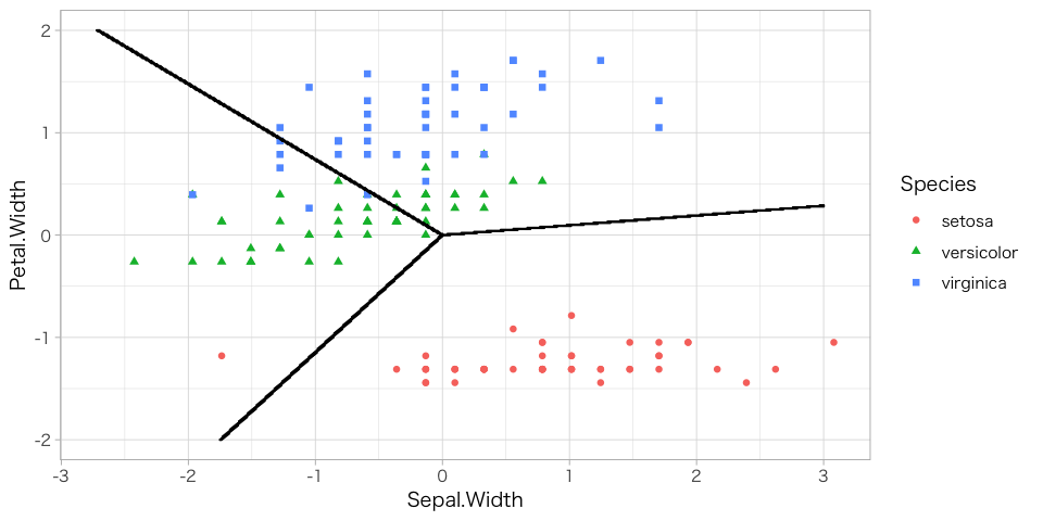
はじパタ6章の二次判別分析で例示されている図を描く方法です。
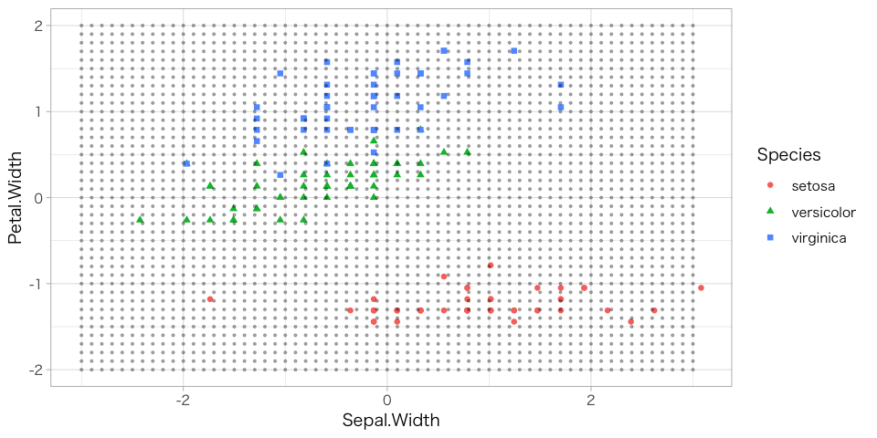
少し泥臭いやり方です。まず網目状に格子を貼り、それぞれの点で識別関数の値を計算します。その上位2つの誤差がe以下の点のみ残し、それ以外は消去するやり方です。
おそらく、このやり方で他の判別分析の図も作れると思います。

コード

qdaのライブラリを使ってないにも関わらず、tidymodels群のパッケージを使っているので見づらいですが。。。

library(tidyverse)
library(tidymodels)

df = iris %>% select(contains("Width"),'Species')

data = df %>% recipe(Species ~.)  %>% step_center(all_predictors()) %>% step_scale(all_predictors()) %>%step_dummy(Species, one_hot = T)  %>% prep(df) %>% bake(df) 

X = data[,c(1,2)] %>% as.matrix
T = data[,-c(1,2)] %>% as.matrix
W = solve(t(X)%*%X) %*% t(X) %*% T

check_border = function(v,e){
    v_order = sort(v,decreasing = TRUE)
    v_order[1]-v_order[2] < e
}
mesh = crossing(seq(-3,3,by=.01),seq(-2,2,.01)
flag = mesh %>% as.matrix) %*% W %>% t %>% as.tibble %>% map_lgl(~check_border(.,.005)) 
border = mesh %>% filter(flag %>% t) %>% rename_all(~c('x','y')) 

df %>% recipe(Species ~.)  %>% step_center(all_predictors()) %>% step_scale(all_predictors())  %>% prep(df) %>% bake(df) %>%
ggplot(aes(x=Sepal.Width,y=Petal.Width)) + geom_point(aes(color=Species, shape=Species)) + geom_point(data=border,aes(x,y),size=.01)