scipy.stats: コルモゴロフ・スミルノフ検定 kstest

from scipy.stats import kstest

kstest(rvs, cdf, args=(), N=20, alternative='two-sided', mode='auto')

★ 1 つの連続変数の分布（分布関数 $F(x)$）が特定の分布関数 $G(x)$ と同じかどうかの 1 標本検定
★ 2 つの連続変数の分布（分布関数 $F_1(x)$，$F_2(x)$）が同じかどうかの 2 標本検定

引数

rvs : 配列，文字列，関数
- 確率変数の観察値の一次元配列（ベクトル）
- 関数（キーワード引数 size を持つこと）
- 文字列の場合は scipy.stats での関数名（乱数生成のために使われる）
cdf : 配列，文字列，関数
- 確率変数の観察値の一次元配列（　この場合は rvs も一次元配列で，2 標本検定が行われる）
  関数（累積密度関数 cdf を計算する）
- 文字列の場合は scipy.stats での関数名（累積密度関数 cdf を計算する）
args : tuple, sequence, optional
rvs または cdf が文字列または関数の場合の引数
N : int, optional
rvs が文字列または関数のときの発生させる乱数の個数。デフォルトは 20 個。
alternative : {'two-sided', 'less', 'greater'}, optional
検定種別。デフォルトは
- 'two-sided' : 両側検定（デフォルト）$F(x) \neq G(x)$
- 'less' : 片側検定 $F(x) \lt G(x)$
- 'greater' : 片側検定 $F(x) \gt G(x)$
mode : $p$ 値の計算に使われる分布を指定する。
- 'auto' : 他の 2 つの指定のいずれかを使う。
- 'exact' : 検定統計量の正確な分布を使う。
- 'asymp': 検定統計量の漸近分布を使う。

他に ks_1samp と ks_2samp があり，それぞれ 1 標本検定，2 標本検定に対応しているが，引数の内容が若干異なっている。

以下の例題は，R の ks.test の example をやってみる。

例題1:　以下の x と y の分布は等しいといえるだろうか?

> x <- rnorm(50)
> y <- runif(30)
> # Do x and y come from the same distribution?
> ks.test(x, y)
> # D = 0.5933, p-value = 1.214e-06

R で発生させたデータを小数点以下 5 桁で Python に持ってくる。

import numpy as np

x = np.array([
       -1.72376,  0.16178, -0.38592,  0.46489,  0.20133, -1.07218,
       -0.04628, -0.49006, -1.29331,  1.39032, -0.1654 , -1.25657,
       -1.66495, -1.22303,  0.11865,  1.2981 ,  2.43068,  0.44305,
        1.01402,  0.56233, -0.07245,  0.74345, -0.96341,  0.77764,
        1.08929,  1.27639,  0.15179, -0.77254,  0.32772, -0.38812,
       -0.47191,  1.63473,  0.10018, -0.52611, -0.50285, -0.21219,
       -0.2901 ,  0.36465, -0.04853, -0.5499 , -0.8373 , -0.39296,
       -0.1728 , -0.55886, -0.90228, -0.52521,  1.74589, -0.88553,
       -1.36538,  0.61068])
y = np.array([
       0.58012, 0.04539, 0.29521, 0.21106, 0.20044, 0.42524, 0.62587,
       0.77392, 0.56537, 0.26077, 0.45016, 0.97627, 0.09354, 0.47203,
       0.57412, 0.76597, 0.93886, 0.92557, 0.89609, 0.50679, 0.76719,
       0.96471, 0.25184, 0.48612, 0.78057, 0.46438, 0.87383, 0.75838,
       0.97611, 0.58732])

from scipy.stats import kstest
kstest(x, y)

KstestResult(statistic=0.5933333333333334, pvalue=1.2135463929420083e-06)

結論:　$p < 0.0001$ なので，有意水準 5% で帰無仮説は棄却される。すなわち，2 つのデータの分布は異なる。

なお，x は標準正規分布，y は一様分布に従う乱数であった。

例題2:

> ks.test(x+2, "pgamma", 3, 2) # two-sided, exact
> # D = 0.3099, p-value = 9.182e-05

kstest(x+2, 'gamma', args=(3, 0, 1/2), mode='exact')

KstestResult(statistic=0.3099256355801757, pvalue=9.180979163496784e-05)

> ks.test(x+2, "pgamma", 3, 2, exact = FALSE) # asymptotic
> # D = 0.3099, p-value = 0.0001347

kstest(x+2, 'gamma', args=(3, 0, 1/2), mode='asymp')

KstestResult(statistic=0.3099256355801757, pvalue=0.00013472932686076826)

> ks.test(x+2, "pgamma", 3, 2, alternative = "gr")
> # D^+ = 0.0094, p-value = 0.9851

kstest(x+2, 'gamma', args=(3, 0, 1/2), mode='exact', alternative='greater')

KstestResult(statistic=0.009394828748738045, pvalue=0.9851446952481949)

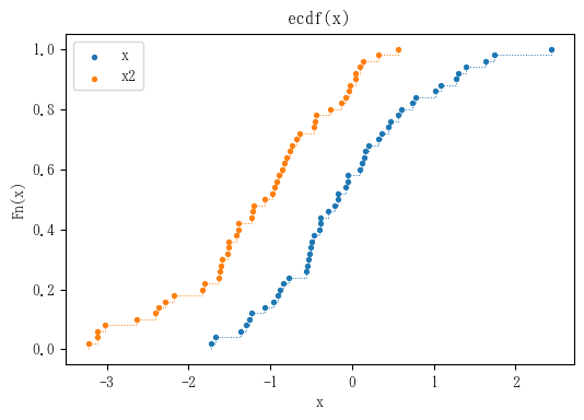
例題3:

> x2 <- rnorm(50, -1)
> plot(ecdf(x), xlim = range(c(x, x2)))
> plot(ecdf(x2), add = TRUE, lty = "dashed")

x2 = np.array([
    -1.20293, -2.28527, -3.01649, -0.64388, -1.069, -0.97615, -1.38786, 
    -0.943, -0.85573, 0.0992, -0.92018, -0.83062, -0.7611, -0.26655, 
    -0.46294, -1.38785, -0.07543, 0.3233, -0.03589, -1.42002, -1.61768, 
    -1.50459, -2.63877, -0.8061, -0.43423, -3.10982, -1.23428, -0.72625, 
    -1.62309, 0.13181, -2.36041, -0.446, 0.55993, -0.02916, 0.04785, 
    -2.40704, -1.58485, -1.51846, -0.67458, -1.50454, 0.0451, -0.89554, 
    -1.59722, -1.82615, -3.2236, -0.13407, -2.17628, -1.2137, -1.80607, 
    -3.11688])

# fit an empirical cdf to a bimodal dataset
import matplotlib.pyplot as plt
from statsmodels.distributions.empirical_distribution import ECDF
# fit a cdf
ecdf = ECDF(x)
ecdf2 = ECDF(x2)
plt.figure(figsize=(6, 4), dpi=100)
plt.scatter(ecdf.x, ecdf.y, s=8)
plt.scatter(ecdf2.x, ecdf2.y, s=8)
plt.legend(['x', 'x2'])
plt.step(ecdf.x, ecdf.y, where='post', linewidth=0.7, linestyle=':')
plt.step(ecdf2.x, ecdf2.y, where='post', linewidth=0.7, linestyle=':')
plt.xlabel('x')
plt.ylabel('Fn(x)')
plt.title('ecdf(x)')
plt.show()

> t.test(x, x2, alternative = "g") # Welch
> # t value = 5.8304, df = 97.846, p-value = 3.56e-08

from scipy.stats import ttest_ind
ttest_ind(x, x2, equal_var=False, alternative='greater')

Ttest_indResult(statistic=5.8303998209331205, pvalue=3.560046700814859e-08)

> wilcox.test(x, x2, alternative = "g") # 連続性の補正あり
> # W = 1964, p-value = 4.355e-07

from scipy.stats import ranksums
ranksums(x, x2, alternative='greater')

RanksumsResult(statistic=4.9221873910763785, pvalue=4.279110256255732e-07)

ranksums に連続性の補正はないが，R で連続性の補正なしの結果と一致

> ks.test(x, x2, alternative = "l")
> # D^- = 0.48, p-value = 6.934e-06

alternative = "l" を指定するところに注意（上の 2 つの検定では "g" を指定した）

kstest(x, x2, alternative='less')

KstestResult(statistic=0.48, pvalue=6.933942843680038e-06)

例題4:

> ks.test(c(1, 2, 2, 3, 3), c(1, 2, 3, 3, 4, 5, 6), exact = TRUE)
> # D = 0.4286, p-value = 0.2424

検定統計量はあっているのだが，$p$ 値が違う。

kstest([1, 2, 2, 3, 3], [1, 2, 3, 3, 4, 5, 6], mode='exact')

KstestResult(statistic=0.42857142857142855, pvalue=0.5454545454545454)