Scikit learn 識別器のいろいろ

機械学習において、どのアルゴリズムを使うべきかの指針として、scikit learn のアルゴリズムチートシートを紹介した。その中の識別器(Classification)だけを見ても、たくさんアルゴリズムが用意されている。本記事では、各識別器がどんなふうに識別境界を決めるのか、直感的にわかるように、比較してみる。

やったこと

• 基本的には、Scikit learn の ExampleにあるClassifier comparisonを再現
• 生成したデータセットを使って、Scikit learnにある識別器を比較
• 各識別器の識別境界を視覚的に確かめる

注意

実際のデータセットでは必ずしも、今回の例のようにはなるとは限らないので、あくまで参考。
特に高次元データを扱う場合は、ナイーブベイズや線形サポートベクターマシンなどの比較的単純な識別器でも識別できたりする。複雑な識別器を使うよりも汎化性が高く、有用なことが多いらしい。

使用する識別器の種類

7通りの識別器で実験。

• k近傍法
• サポートベクターマシン（線形）
• サポートベクターマシン（ガウシアンカーネル）
• 決定木
• ランダムフォレスト
• Adaブースト
• ナイーブベイズ
• 線形判別分析
• 二次判別分析

サンプルデータ

Sckit learnの分類問題用のデータ生成機能を使う。性質の異なる次の３種類のデータセットを使用。

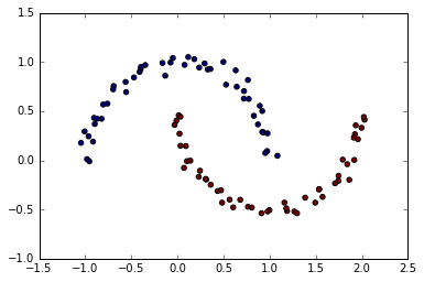
1. 2つの半円状の2次元データ（線形識別不可）
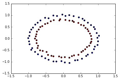
2. 2つの同心円上の2次元データ（線形識別不可）
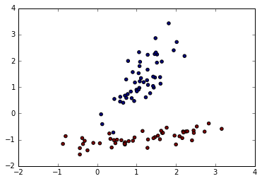
3. 線形識別可能なデータセット

2つの半円状の2次元データ（線形識別不可）

make_moonで生成。グラフの点の色はラベルを示す。

X, y = make_moons(noise = 0.05, random_state=0)

2つの同心円上の2次元データ（線形識別不可）

make_circleで生成。

X, y = make_circles(noise = 0.02, random_state=0)

線形識別可能なデータセット

make_classificationで生成。make_classificationはこちらの解説記事がわかりやすい。ありがとうございます。

• scikit-learnを用いたサンプルデータ生成

以下の例では、２次元の特徴量を有する入力データセットXと、２属性のラベルデータセットyが、それぞれ100個生成される。

X, y = make_classification(n_features=2, n_redundant=0, n_informative=2,
                           random_state=5, n_clusters_per_class=1, n_samples=100, n_classes=2)

結果

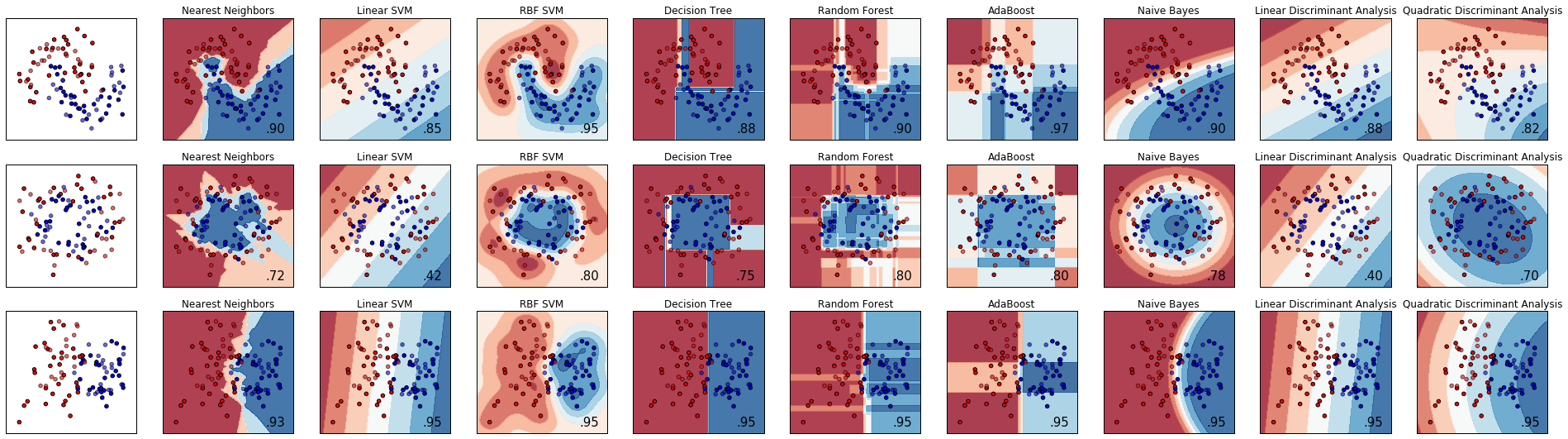
出力結果がこちら。一番左の列が元データ、左から2番目以降は列ごとに、異なる識別器での識別境界を示す。上段が半円データセット、中段が同心円データセット、下段が線形分離可能なデータセットを用いた場合。各グラフ内の右下に表示されている数字はモデルの精度を示す評価値。識別器ごとの識別境界の引き方の特徴がよくわかる。

（参考）コード

コメントを日本語で追記した以外は、基本的にソースClassifier comparisonのまんま。

# -*- coding: utf-8 -*-
import numpy as np
import matplotlib.pyplot as plt
%matplotlib inline
from matplotlib.colors import ListedColormap
from sklearn.cross_validation import train_test_split
from sklearn.preprocessing import StandardScaler
from sklearn.datasets import make_moons, make_circles, make_classification
from sklearn.neighbors import KNeighborsClassifier
from sklearn.svm import SVC
from sklearn.tree import DecisionTreeClassifier
from sklearn.ensemble import RandomForestClassifier, AdaBoostClassifier
from sklearn.naive_bayes import GaussianNB
from sklearn.discriminant_analysis import LinearDiscriminantAnalysis
from sklearn.discriminant_analysis import QuadraticDiscriminantAnalysis
h = .02  # step size in the mesh

names = ["Nearest Neighbors", "Linear SVM", "RBF SVM", "Decision Tree",
         "Random Forest", "AdaBoost", "Naive Bayes", "Linear Discriminant Analysis",
         "Quadratic Discriminant Analysis"]
classifiers = [
    KNeighborsClassifier(3),
    SVC(kernel="linear", C=0.025),
    SVC(gamma=2, C=1),
    DecisionTreeClassifier(max_depth=5),
    RandomForestClassifier(max_depth=5, n_estimators=10, max_features=1),
    AdaBoostClassifier(),
    GaussianNB(),
    LinearDiscriminantAnalysis(),
    QuadraticDiscriminantAnalysis()]


# ランダムな2クラス識別問題用のデータを生成
# 2次元の入力データXと、2クラスのラベルデータyをそれぞれ100サンプル生成
X, y = make_classification(n_features=2, n_samples=100, n_redundant=0, n_informative=2,
                           random_state=1, n_clusters_per_class=1, n_classes=2)
rng = np.random.RandomState(0) # 乱数生成器のクラス、数字はシードなので何でもよい
X += 2 * rng.uniform(size=X.shape) # 元のデータを加工
linearly_separable = (X, y) # 線形識別可能なデータセット

datasets = [make_moons(noise=0.25, random_state=0),
            make_circles(noise=0.2, factor=0.6, random_state=1),
            linearly_separable
            ]

figure = plt.figure(figsize=(27, 9))
i = 1
# 3種類のデータセットでループ
for ds in datasets:
    # データの前処理、トレにーニング用とテスト用にデータセット分割
    X, y = ds
    X = StandardScaler().fit_transform(X) # データを正規化
    X_train, X_test, y_train, y_test = train_test_split(X, y, test_size=.4)

    x_min, x_max = X[:, 0].min() - .5, X[:, 0].max() + .5
    y_min, y_max = X[:, 1].min() - .5, X[:, 1].max() + .5
    xx, yy = np.meshgrid(np.arange(x_min, x_max, h),
                         np.arange(y_min, y_max, h))

    # データセットのみをプロット
    cm = plt.cm.RdBu
    cm_bright = ListedColormap(['#FF0000', '#0000FF'])
    ax = plt.subplot(len(datasets), len(classifiers) + 1, i)
    ax.scatter(X_train[:, 0], X_train[:, 1], c=y_train, cmap=cm_bright) # トレーニング用
    ax.scatter(X_test[:, 0], X_test[:, 1], c=y_test, cmap=cm_bright, alpha=0.6) # テスト用は明るい色で
    ax.set_xlim(xx.min(), xx.max())
    ax.set_ylim(yy.min(), yy.max())
    ax.set_xticks(())
    ax.set_yticks(())
    i += 1

    # 識別器でループ
    for name, clf in zip(names, classifiers):
        ax = plt.subplot(len(datasets), len(classifiers) + 1, i)
        clf.fit(X_train, y_train)
        score = clf.score(X_test, y_test)

        # 決定境界をプロットするため、格子状の各点での推定値を計算。
        if hasattr(clf, "decision_function"):
            Z = clf.decision_function(np.c_[xx.ravel(), yy.ravel()]) # 決定境界からの距離
        else:
            Z = clf.predict_proba(np.c_[xx.ravel(), yy.ravel()])[:, 1] # 確率

        # カラープロット
        Z = Z.reshape(xx.shape)
        ax.contourf(xx, yy, Z, cmap=cm, alpha=.8) # 格子状データ
        ax.scatter(X_train[:, 0], X_train[:, 1], c=y_train, cmap=cm_bright) # トレーニング用データ点
        ax.scatter(X_test[:, 0], X_test[:, 1], c=y_test, cmap=cm_bright, alpha=0.6) # テスト用データ点

        ax.set_xlim(xx.min(), xx.max())
        ax.set_ylim(yy.min(), yy.max())
        ax.set_xticks(())
        ax.set_yticks(())
        ax.set_title(name)
        ax.text(xx.max() - .3, yy.min() + .3, ('%.2f' % score).lstrip('0'),
                size=15, horizontalalignment='right')
        i += 1

figure.subplots_adjust(left=.02, right=.98)
plt.show()