SAS ViyaはAIプラットフォームを提供しています。デモもあるのですが、全体が英語なので利用するまでに躊躇してしまう人も多いかと思います。そこで、Pythonで機械学習パイプラインを利用するまでの流れを紹介します。
利用開始まで
まず SASの開発者サイトにアクセスします。開発者サイトは https://developer.sas.com/home.html です。
そして、 Get started with your SAS Viya Developer Trial を押します。
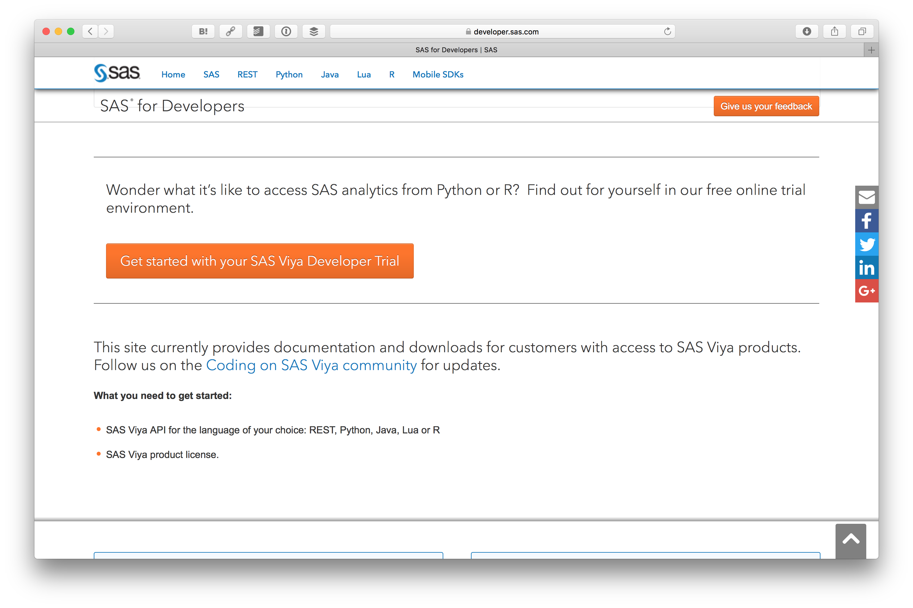
試すためには SAS Profile (SASプロファイル) というのが必要です。まず Create one をクリックします。

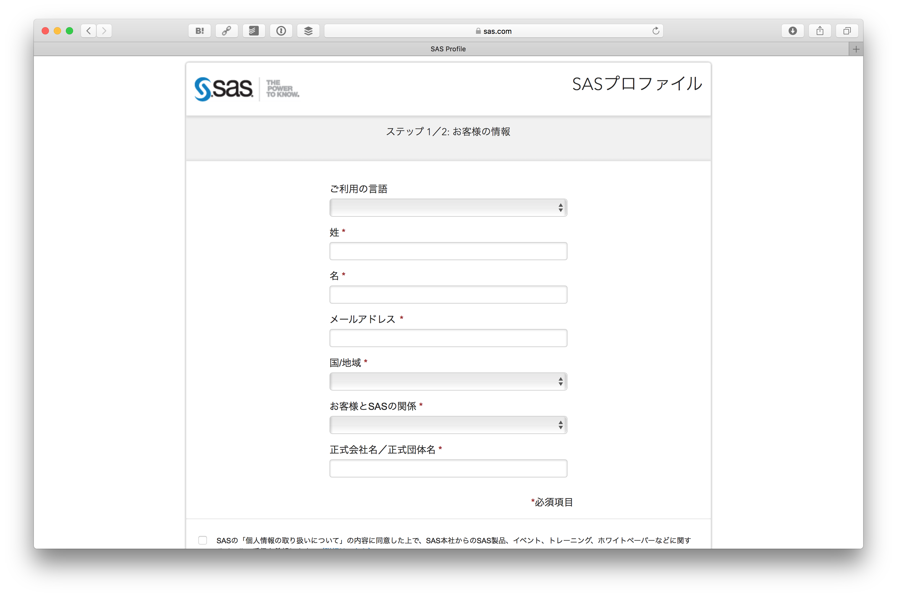
SASプロファイルを登録するをクリックします。

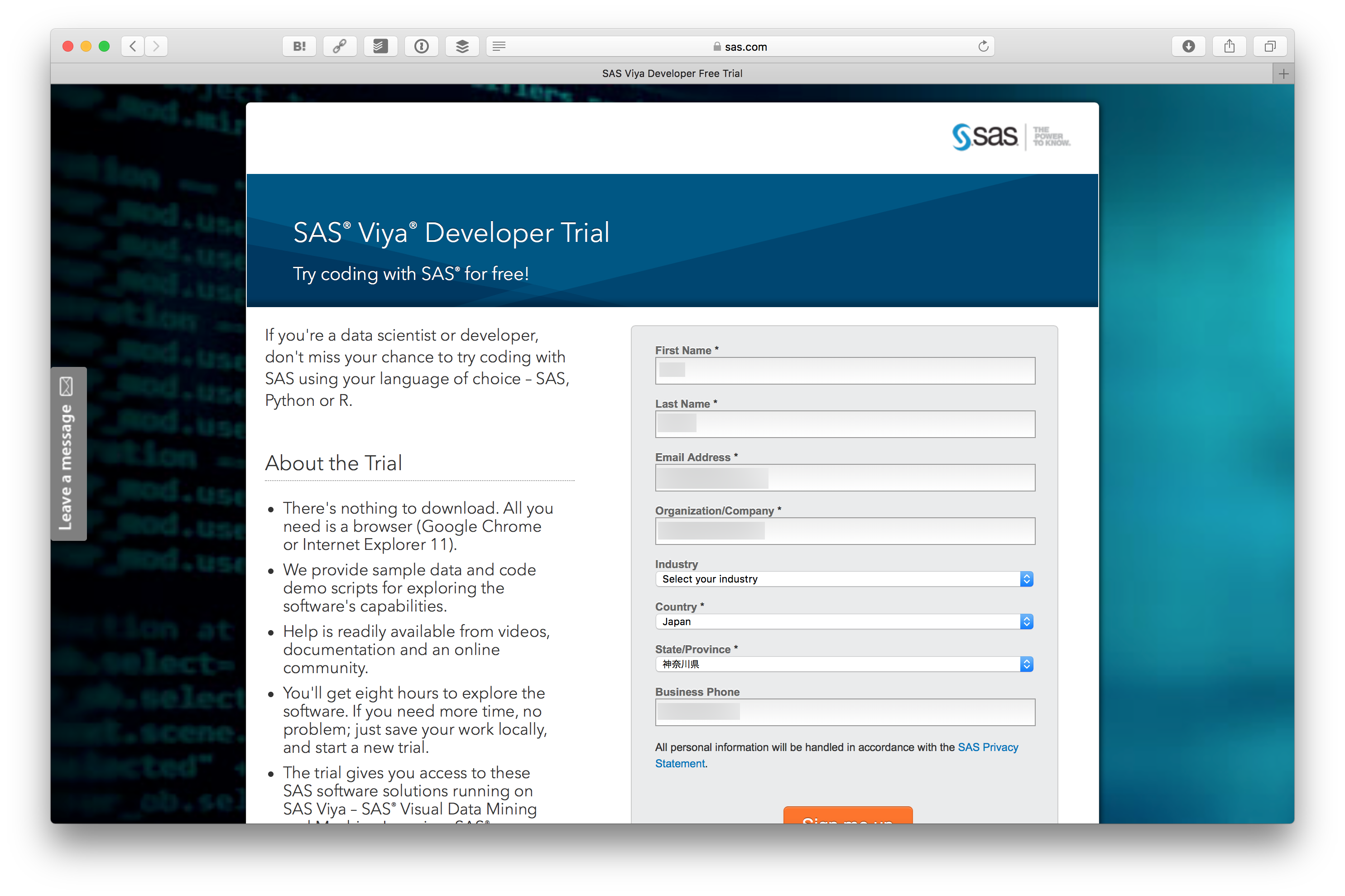
情報を入力します。
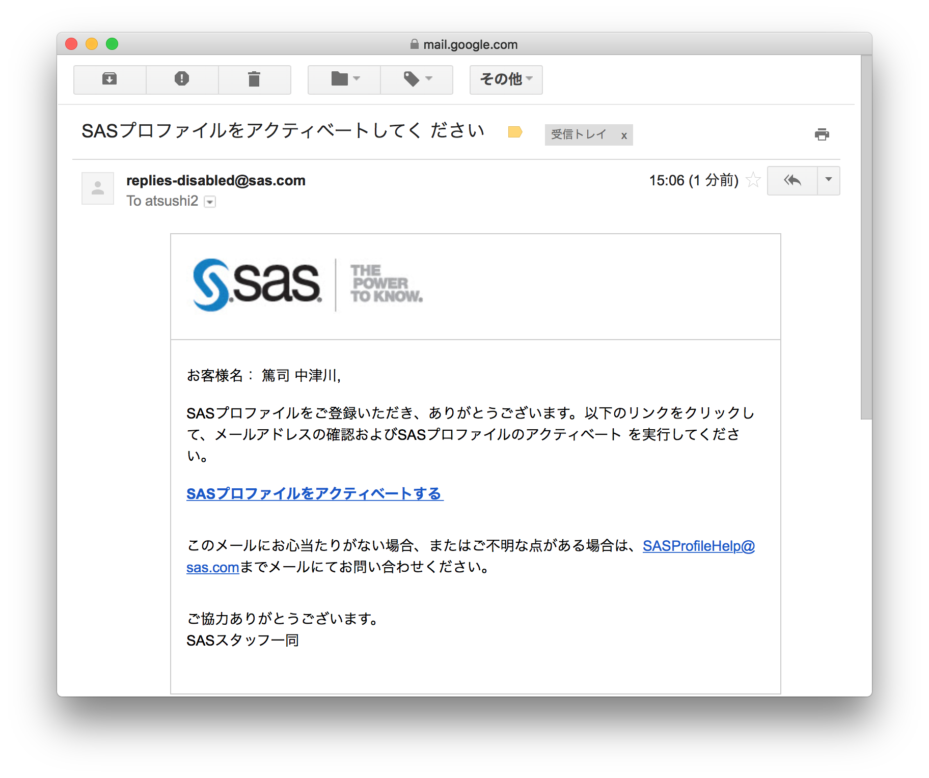
フォームを送信するとメールが送られてきます。
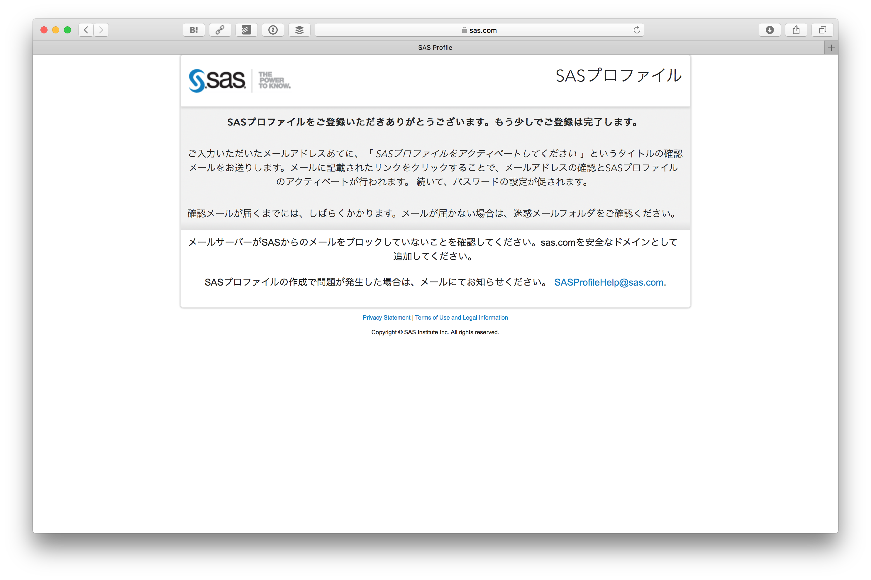
メールに書かれている SASプロファイルをアクティベートする をクリックします。
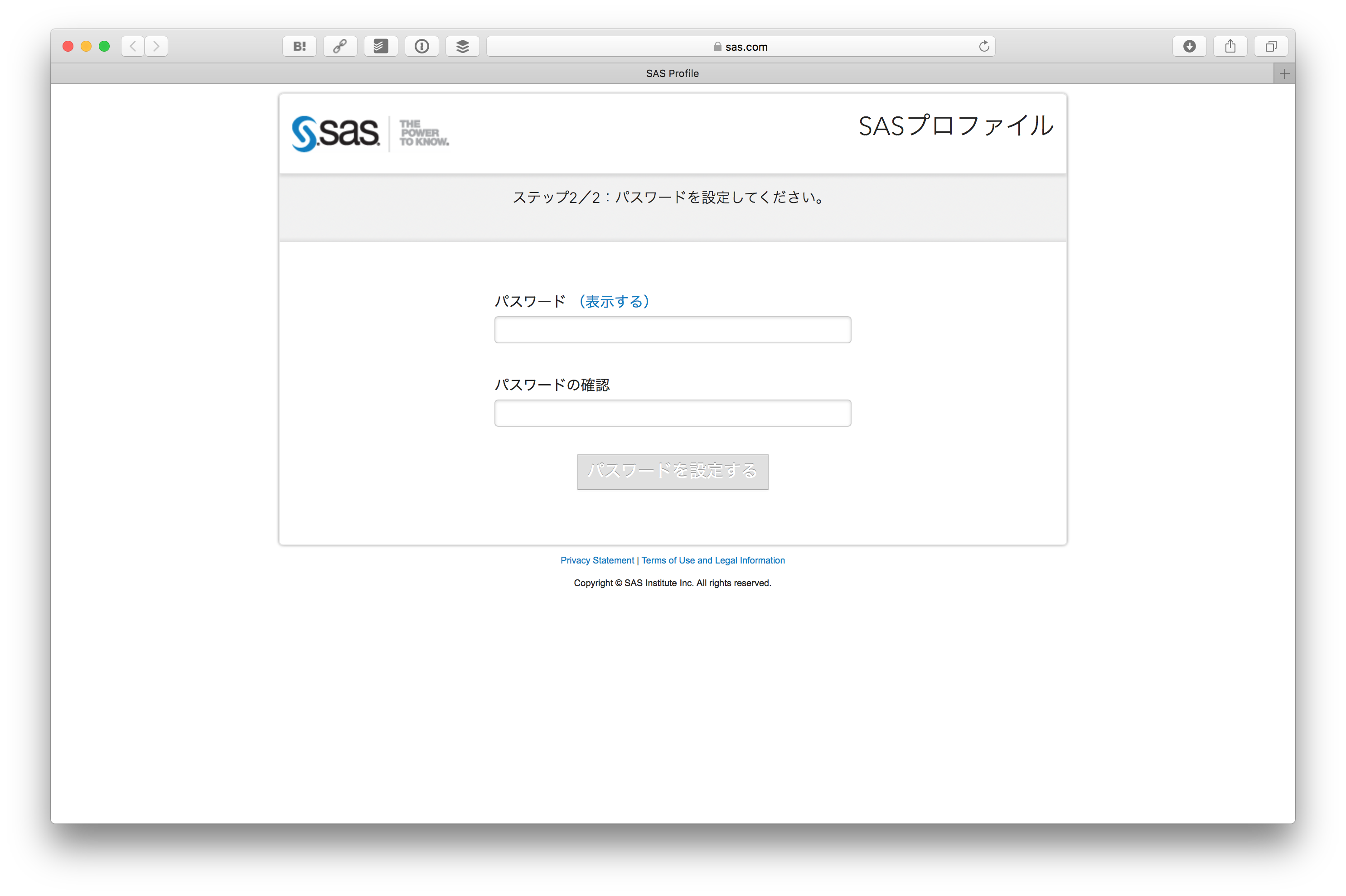
そしてパスワードを設定します。
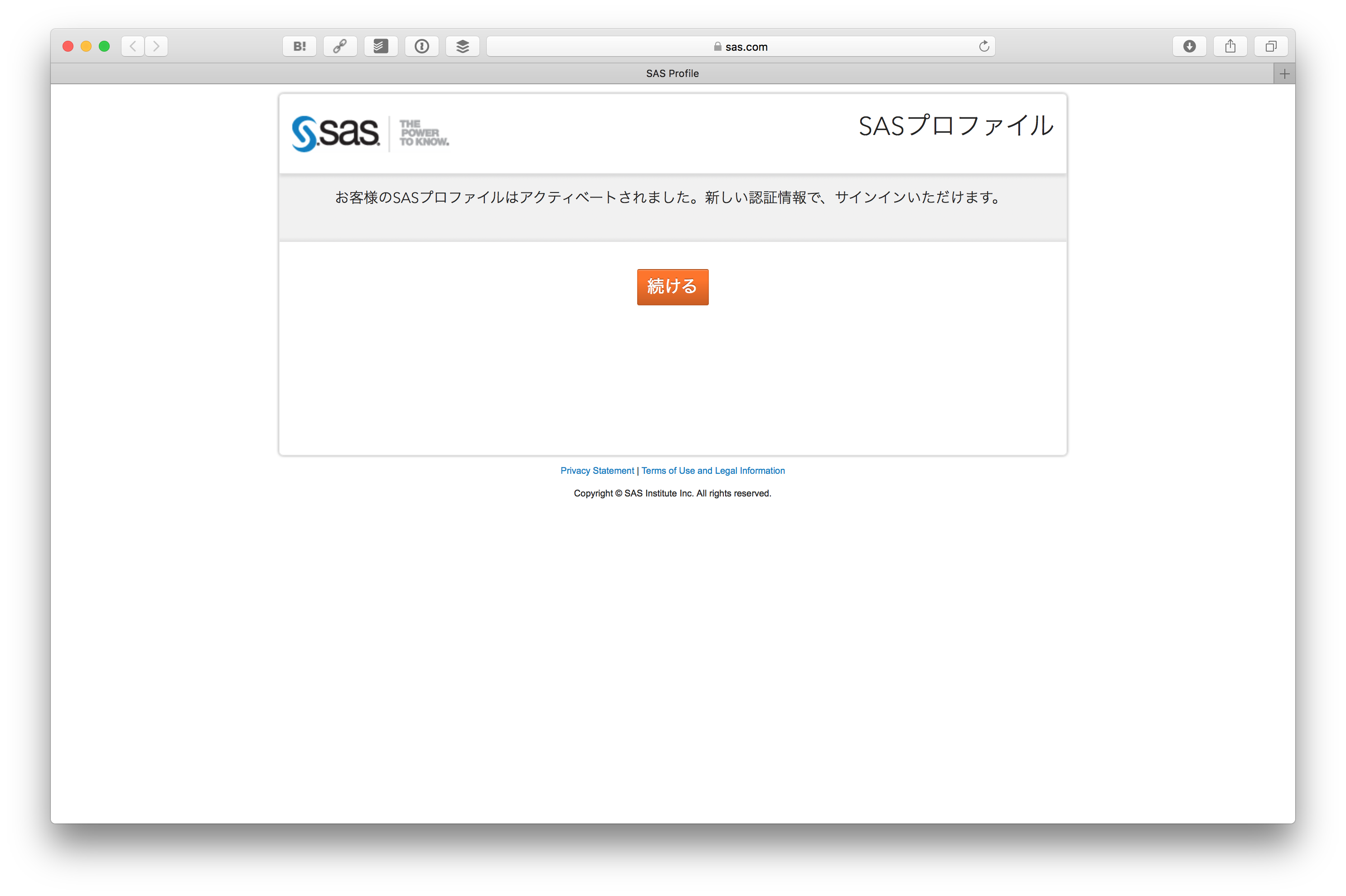
SASプロファイルがアクティベートされます。 続ける をクリックします。
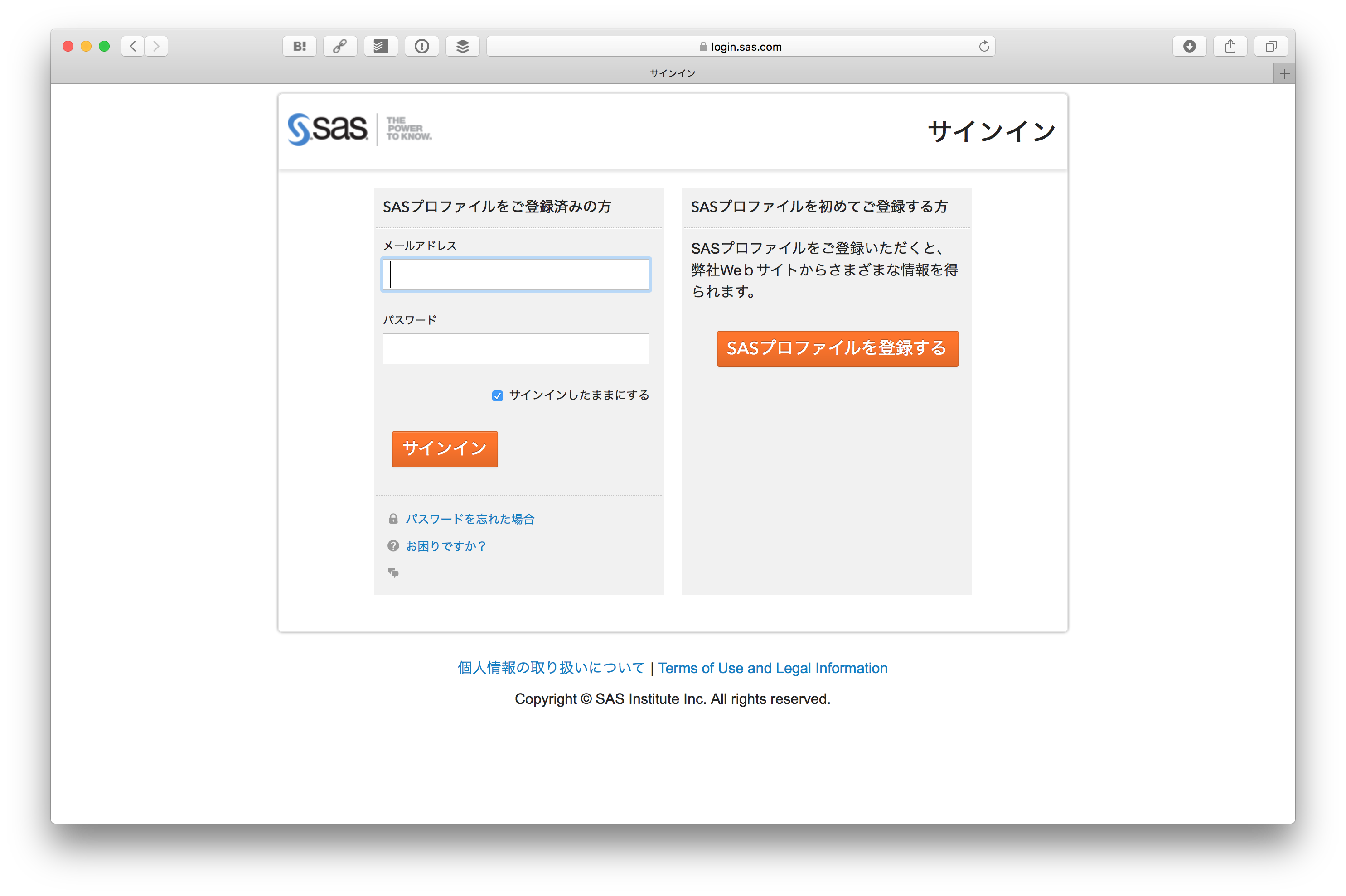
そうすると先ほどの SAS® Viya® Developer Trial の画面に戻ってきますので、 今度はSign In をクリックします。
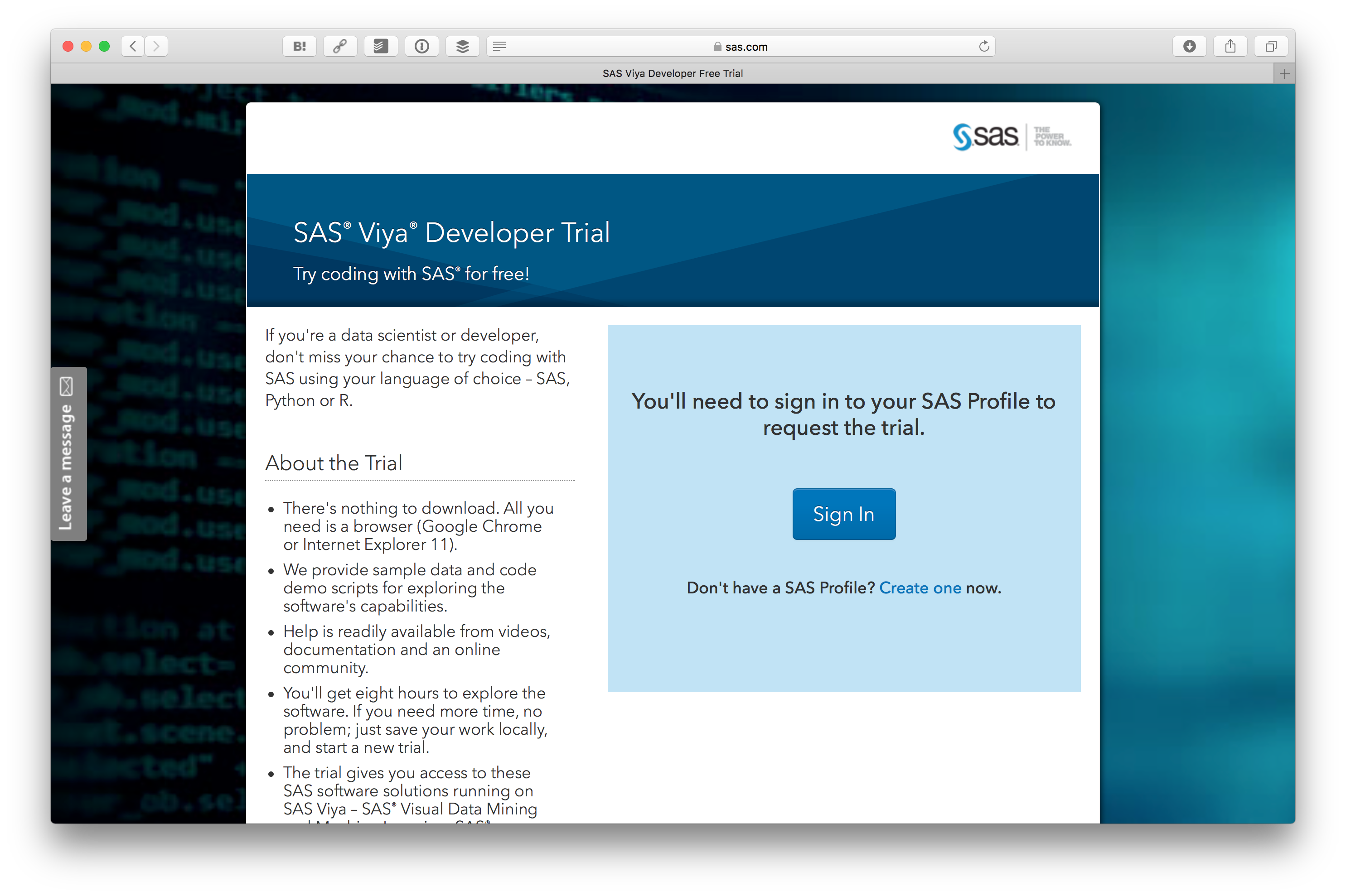
先ほど登録したSASプロファイルのID、パスワードでログインします。
ログインすると SAS® Viya® Developer Trial の画面に戻ってきますが、今回はプロファイルの内容が入力されているはずです。一番下にある Sign me upボタンをクリックします。
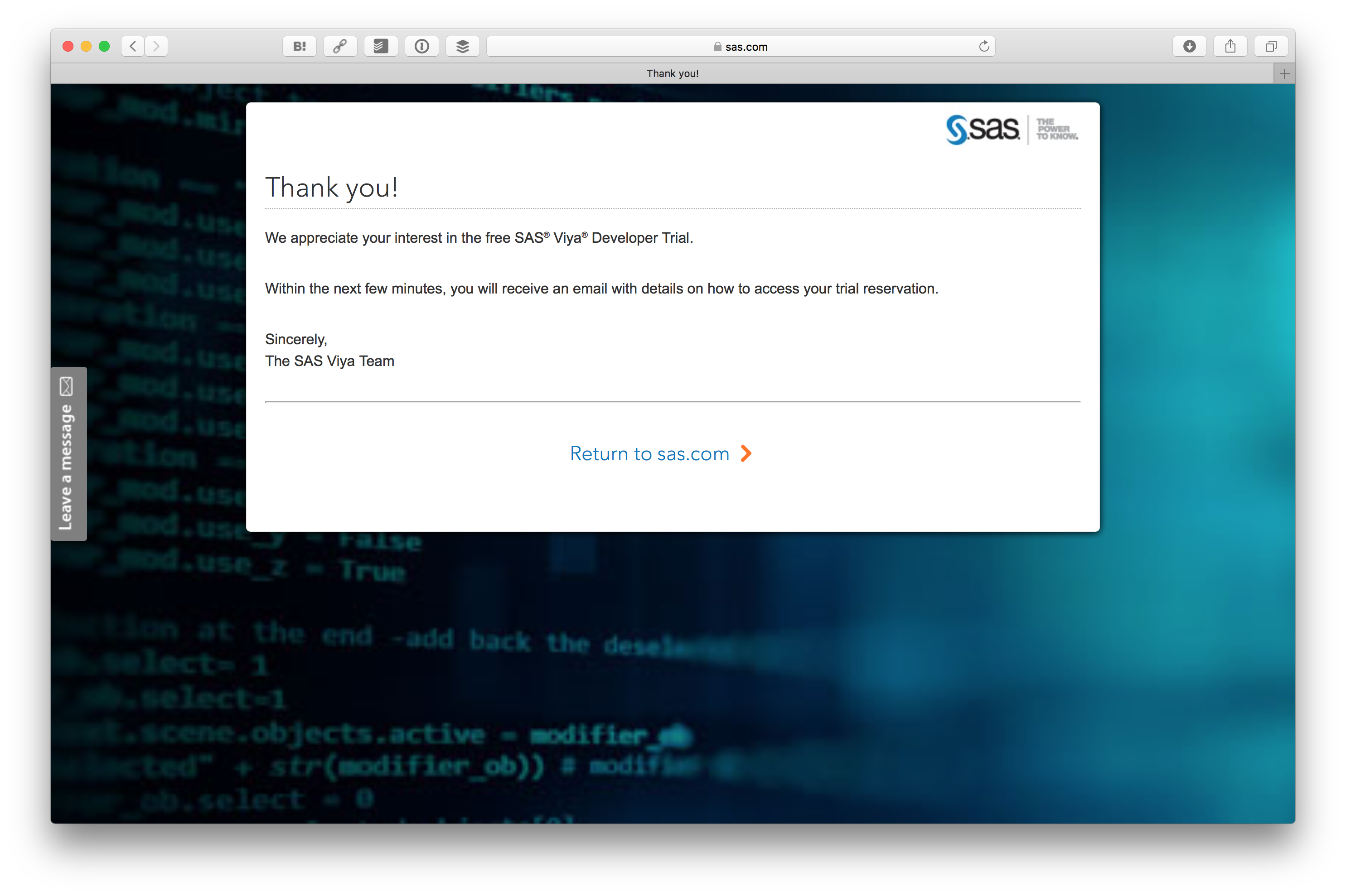
これで SAS® Viya® Developer Trial の申し込みが終わりました。数分後にメールが送られてきます。
送られてきたメールにある Log in to your Trial Portal のリンクをクリックします。

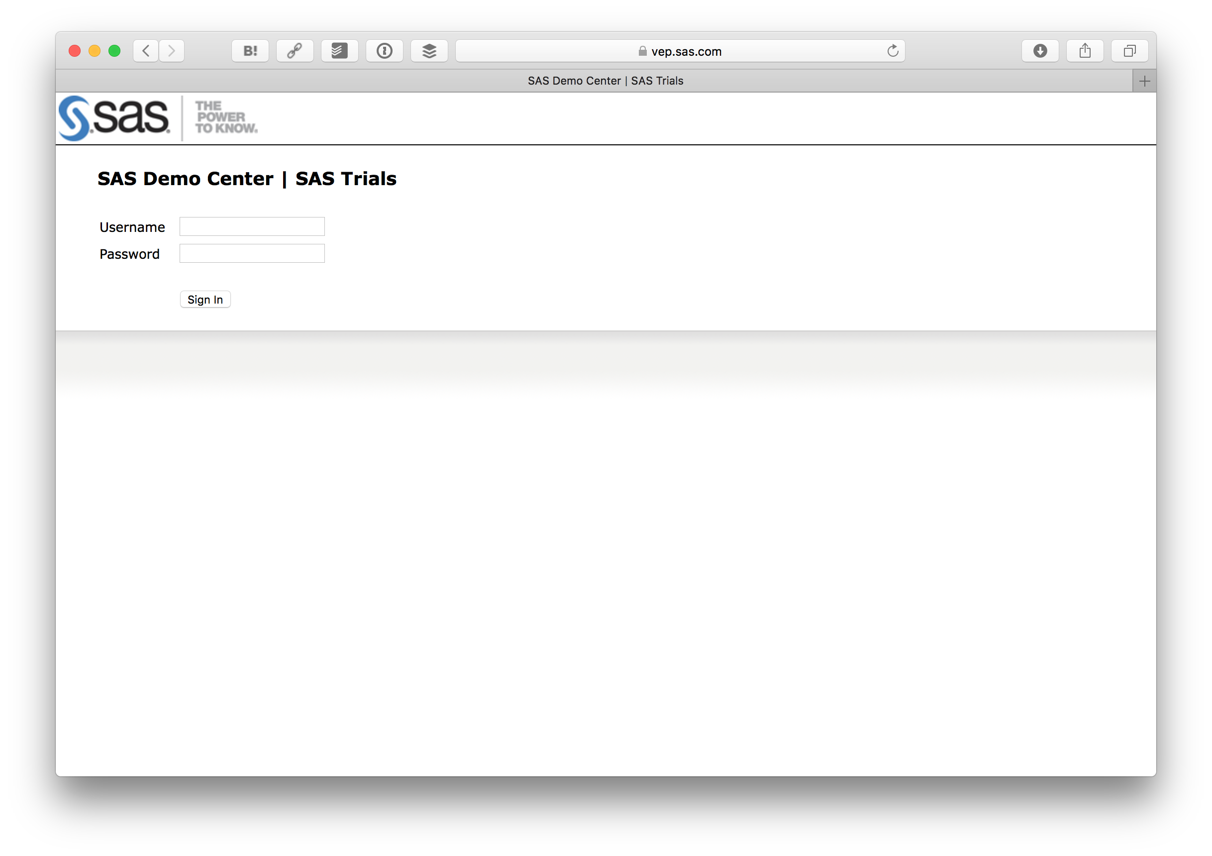
利用規約が表示されますので、問題なければAcceptボタンを押します。
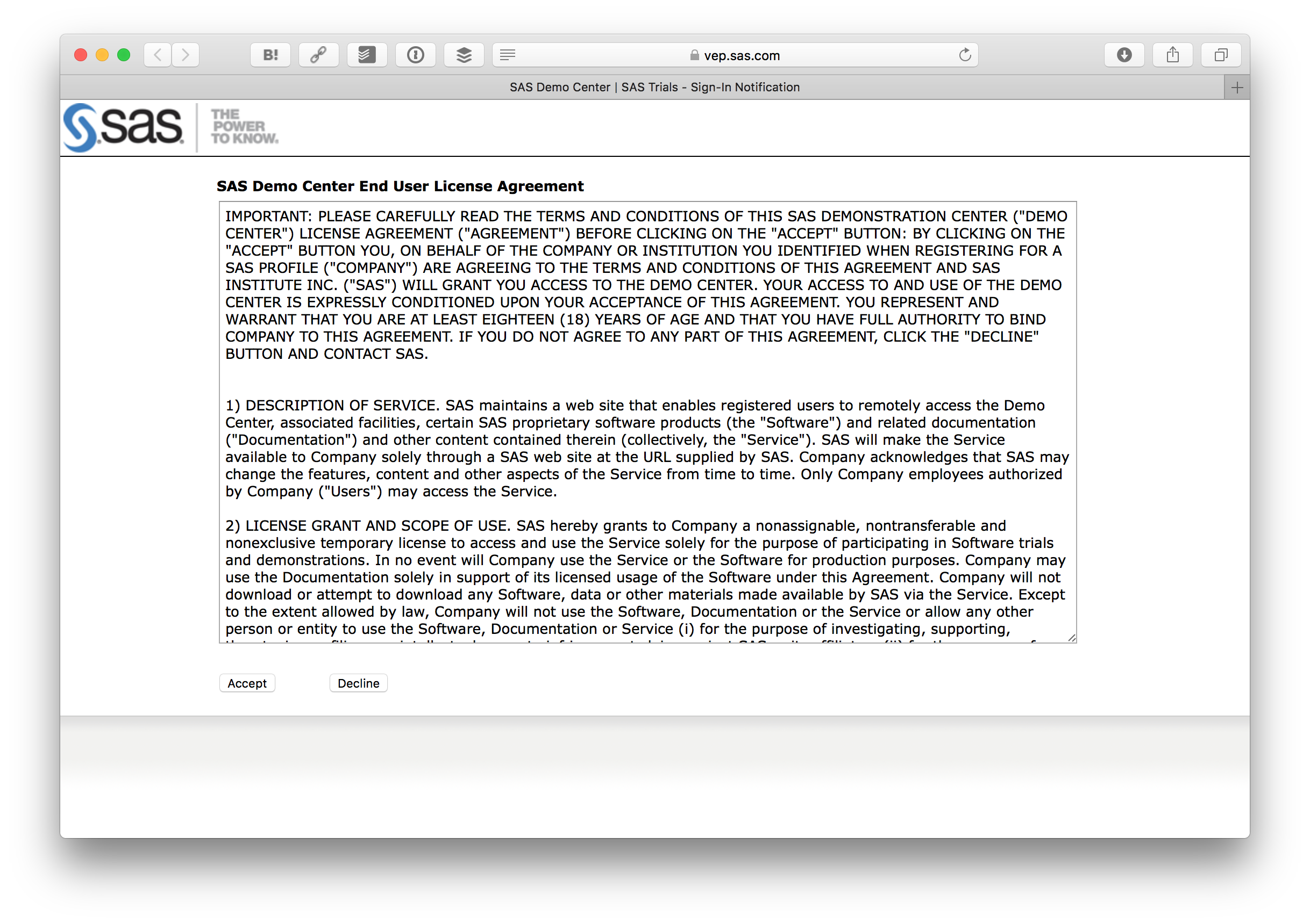
そうするとログインフォームが出るので、先ほど登録したID、パスワードでログインします。
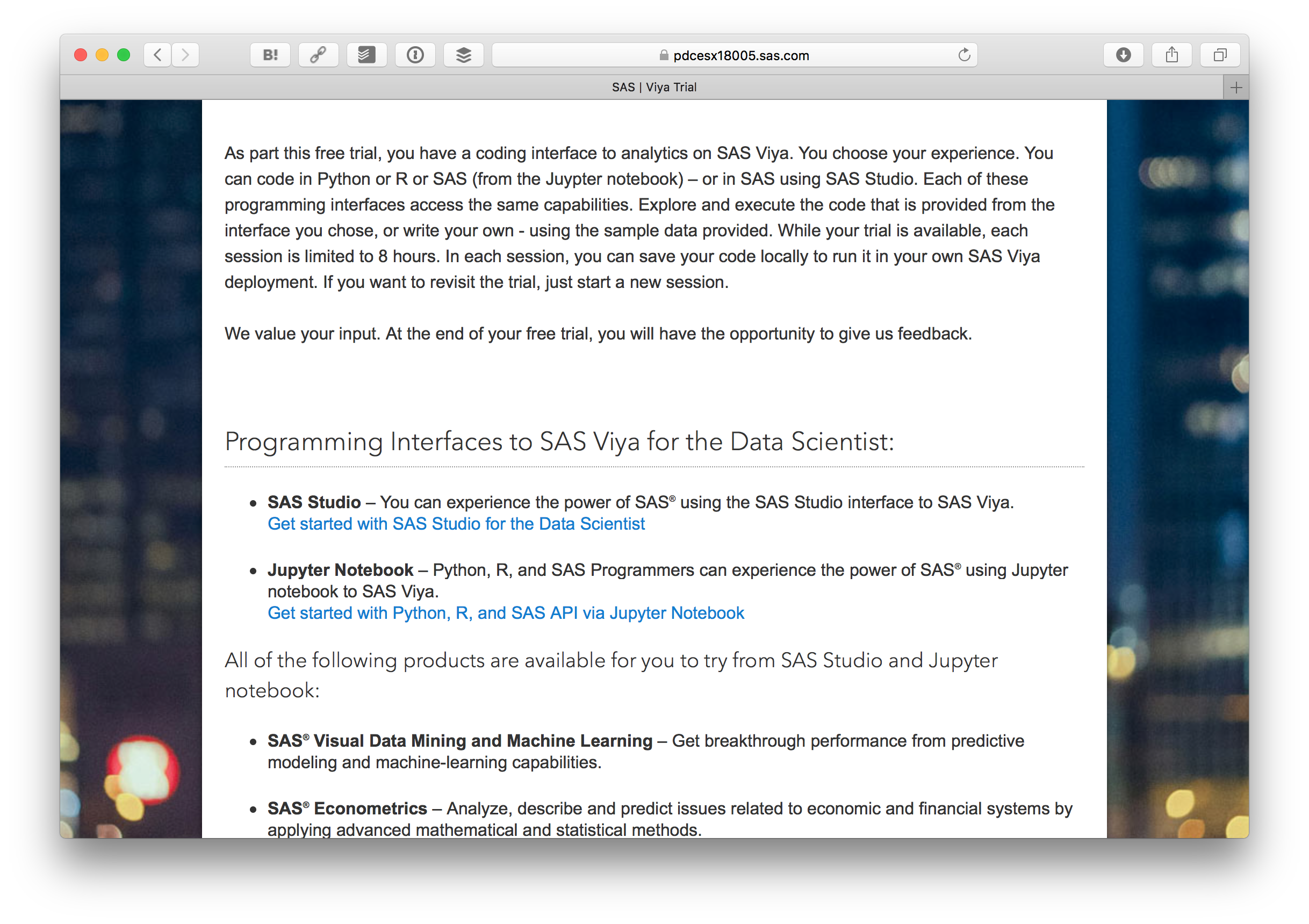
ログインすると Getting Started: SAS® Viya™ Developer Trial が表示されます。
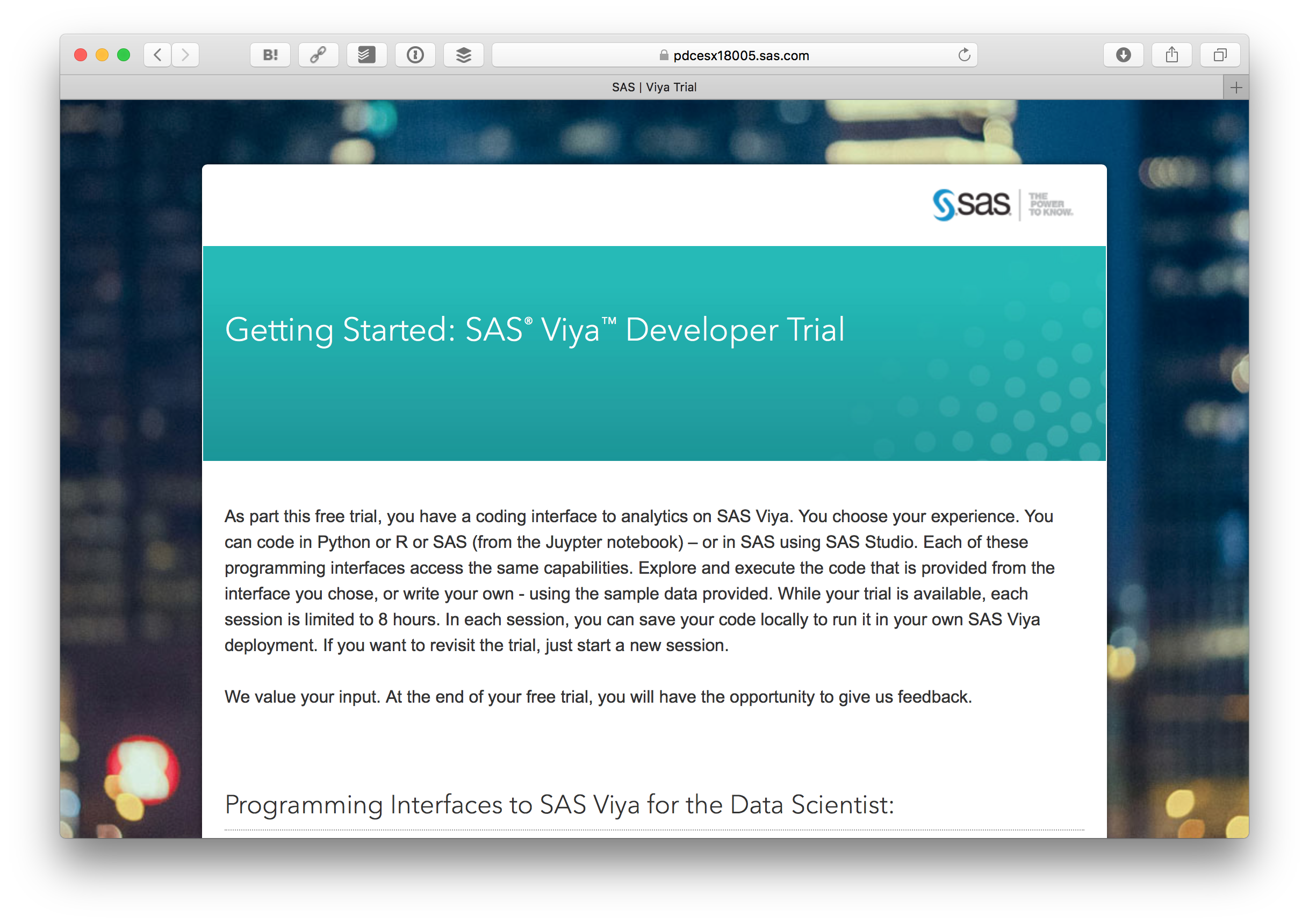
下の方にある Get started with Python, R, and SAS API via Jupyter Notebook をクリックします。
さらに Start My Trial Now をクリックします。
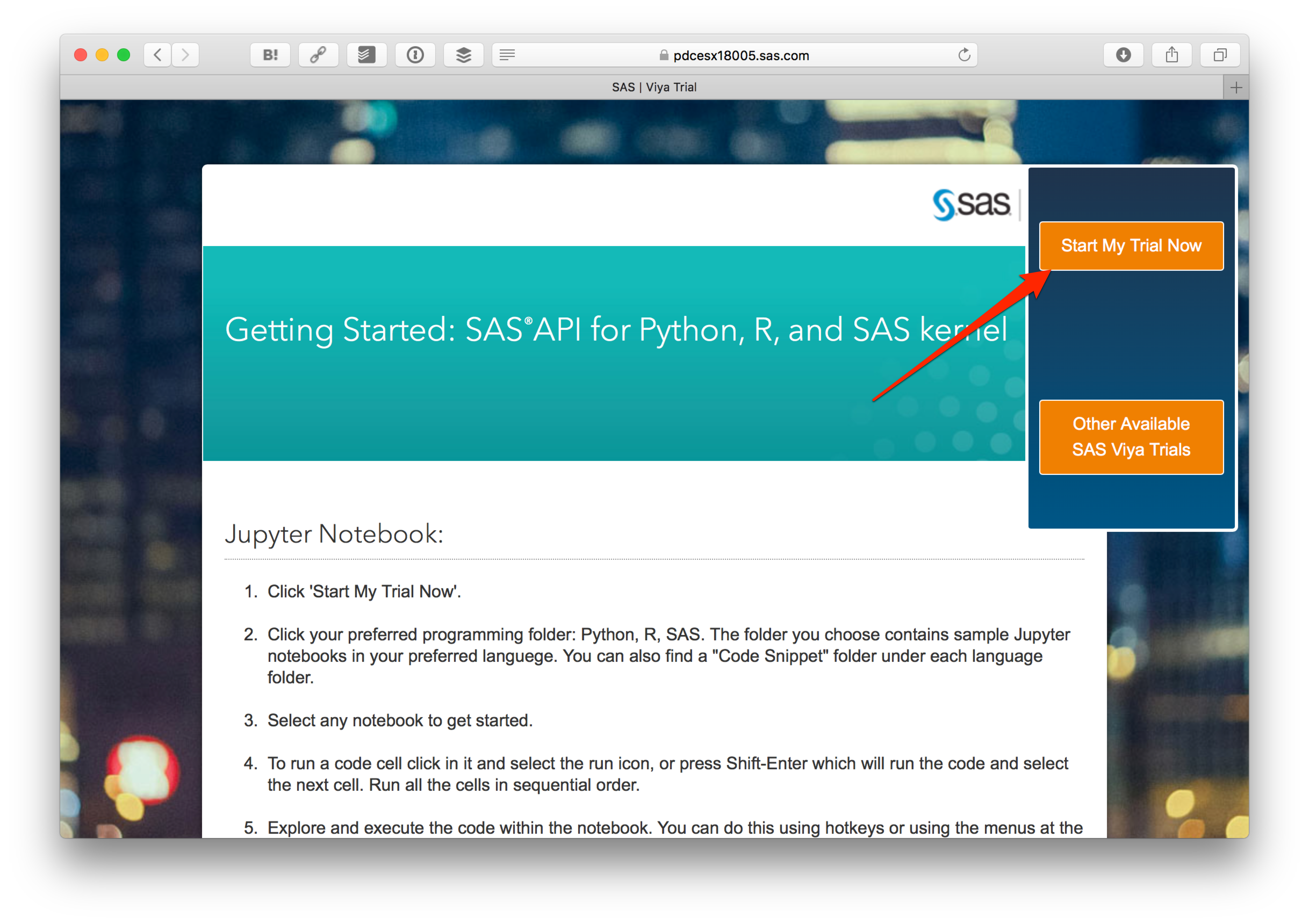
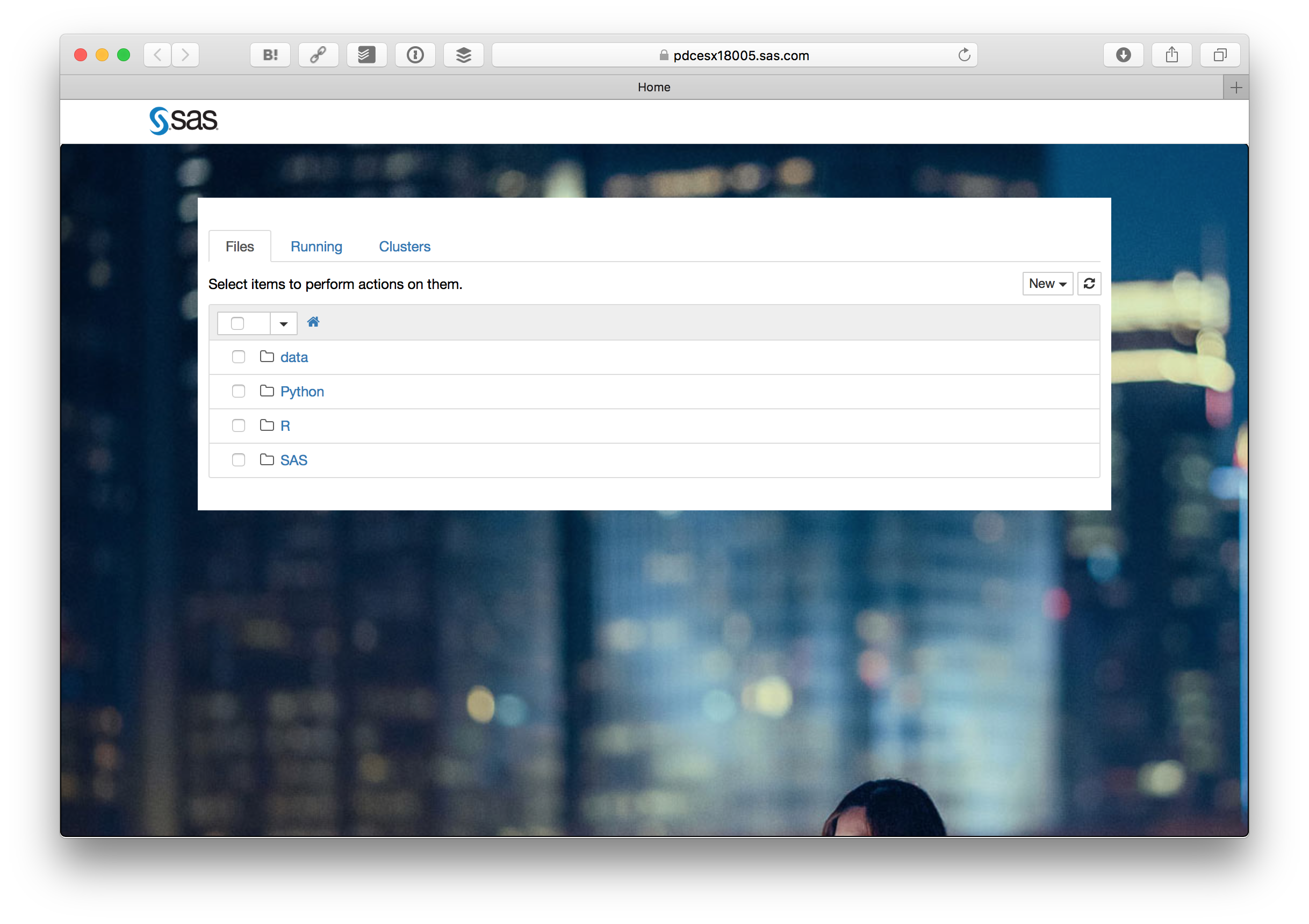
そうすると見慣れたJupyter Notebookの画面が出ます。Pythonフォルダの中にある EmployeeChurnPipefitter.ipynb をクリックします。
ここからは EmployeeChurnPipefitter.ipynb に書かれている内容の意訳です。英語の後に日本語を参考として載せています。
Machine Learning Pipeline: Using Pipefitter with SAS Viya(機械学習パイプライン: SAS ViyaにおけるPipefitterの利用法)
The goal is to supply a uniform set of high-level APIs built on top of SAS 9.4 and SAS Viya that help users create and tune practical machine learning pipelines. The idea is currently applied in open source framework scikit-learn and spark.ml.
このJupyter Notebookの目標はSAS 9.4とSAS Viya上に構築された実用的なパイプラインを作成し、高度かつ統一されたAPIセットを体験します。この手法はオープンソース・フレームワークのscikit-learnとspark.mlで用いられています。
The three primary components used in the workflow are:
このワークフローで使用される主なコンポーネントは次の3つです。
- Transformer (変換器)
- Estimator (推定)
- Pipeline (パイプライン)
Create Connections and Load Data (接続の作成とデータの読み込み)
The PipelineConnection object is a thin wrapper around the saspy and SWAT connection objects. While these objects use very different connection parameters, methods such as read_csv can be normalized between them using this object.
PipelineConnection オブジェクトは、saspyとSWAT接続オブジェクトを扱う薄いラッパーです。これらのオブジェクトはまったく異なる接続パラメータを使用しますが、このオブジェクトを使用して read_csv などのメソッドを扱えるようになります。
import swat
import pipefitter
SAS Viya Version(SAS ViyaのVersion)
cashost='localhost'
casport=5570
casauth='~/.authinfo'

casconn = swat.CAS(cashost, casport, authinfo=casauth, caslib="casuser")
hr_table = casconn.read_csv('../data/HR_comma_sep.csv')
hr_table.head()
hr_table.info()
Pipefitter Classes (Pipefitterクラス)
These classes are agnostic across connection types. They simply proxy all method calls to the appropriate classes in the registered backends. New backends can be registered using the name of the data type of the table object as the key.
これから紹介するクラスは、接続タイプに依りません。利用しているバックエンドの適切なクラスへのすべてのメソッド呼び出しをプロキシします。新しいバックエンドは、テーブルオブジェクトのデータ型の名前をキーとして登録できます。
The SAS Pipefitter project provides a Python API for developing machine learning pipelines. The pipelines are built from stages that perform variable transformation, parameter estimation, and hyperparameter tuning.
「SAS PipeFitter」は、機械学習パイプライン(≒プロセスフロー)を作成するためのPythonのAPIです。機械学習パイプラインとは、変数の変換、パラメータ推定、ハイパーパラメーターのチューニングなどの処理で構成されます。
Estimator(推定器)
from pipefitter.estimator import DecisionTree, DecisionForest, GBTree
Create a DecisionTree object. This object is the high-level object that has no knowledge of CAS or SAS.
DecisionTreeオブジェクトを作成します。 このオブジェクトは、CASまたはSASとは関係のない、高レベルのオブジェクトです。
# params = dict(target='Survived',
#              inputs=['Sex','Age','Fare'],
#              nominals=['Sex', 'Survived'])
params = dict(target = 'left',
              inputs = ['satisfaction_level', 'last_evaluation', 'number_project',
                        'average_montly_hours', 'time_spend_company', 'Work_accident',
                        'promotion_last_5years', 'sales', 'salary'],
              nominals = ['left', 'sales', 'salary', 'promotion_last_5years'])
These are the parameters stored on the DecisionTree object.
これらは DecisionTree オブジェクトに格納されているパラメータです。
dtree = DecisionTree(max_depth=6, **params)
dtree
Run the fit method against the hr_table. This fit method does some parameter validation, then looks up the appropriate sub-package for the table object to locate the correct backend implementation to call. It then creates an instance of that class with the same parameters that the original constructor received. The fit method of that object is then called.
hr_table に対して fit メソッドを実行します。 この fit メソッドは、いくつかのパラメータの検証を行い、指定されたテーブルオブジェクトの適切なサブパッケージを参照して、バックエンド実装の呼び出すメソッドを探します。 次に、元のコンストラクタが受け取ったパラメーターと同じパラメーターを使用して、そのクラスのインスタンスを作成します。最後に生成したインスタンスの fit メソッドを実行します。
Decision Tree Fit and Score of CAS Table(CASテーブルの決定木適合度とスコア)
Using the DecisionTree instance, we'll first run the fit method on the hr_table variable.
DecisionTree インスタンスを使用して、最初に hr_table変数に対して fit メソッドを実行します。
model = dtree.fit(hr_table)
model
vars(model)
**dtree results(dtreeの結果)
The score method can then be called on a table. The model from the fit method was automatically stowed away and is passed to the score method of the real implementation. The output of the underlying CAS action is normalized by the real implementation class and is returned to the user.
テーブル上で score メソッドを呼び出せます。 fit はモデルから自動的に消され、実装されている score メソッドに渡されます。ベースになるCASアクションの出力は、実装クラスによって処理され、ユーザに返されます。
In this case, we are emulating scikit-learn's behavior of returning the misclassification rate.
このケースでは誤分類率を返す scikit-learn の動作をエミュレートしています。
score = model.score(hr_table)
score
Fields from the output can be selected using standard DataFrame techniques. There are a common set of fields for all backends, but other fields may be available depending on what the backend model can produce.
出力にあるフィールドは、標準の DataFrame 技術を使用して選択できます。 すべてのバックエンドに共通のフィールドセットがありますが、バックエンドモデルが生成できるものに応じて他のフィールドを使用できます。
score.loc['MisClassificationRate']
Decision Forest(デシジョン フォレスト)
rf = DecisionForest(**params)
rfmodel = rf.fit(hr_table)
rfmodel
rfmodel.score(hr_table)
Gradient Boosting one liner(一行で記述する場合)
GBTree(**params).fit(hr_table).score(hr_table)
Generic Imputer (一般的な代入)
Imputing can also be done using classes that work with multiple backends.
複数のバックエンドで動作するクラスを使用して、代入を行えます。
from pipefitter.transformer import Imputer
imp = Imputer(value=Imputer.MODE)
imp
hr_table.info()
datamode = imp.transform(hr_table)
datamode.info()
datamean = Imputer(value=Imputer.MEAN).transform(datamode)
datamean.info()
datamean.head()
Pipeline(パイプライン)

Defining the Pipeline(パイプラインの定義)
Each component of a pipeline consists of tuples that specify a label for the component and a class instance for that step in the pipeline.
パイプラインの各コンポーネントは、コンポーネントのラベルとパイプラインの中にある各ステップのクラスインスタンスという組み合わせで構成されています。
from pipefitter.pipeline import Pipeline
from pipefitter.transformer import Imputer

mode_imputer = Imputer(value=Imputer.MODE)
mean_imputer = Imputer(value=Imputer.MEAN)
Now we define the estimators. In this case, we'll use the same parameters for all of them.
ここで 推定器を定義します。この場合、すべて同じパラメータを使用します。
from pipefitter.estimator import DecisionTree, DecisionForest, GBTree
params = dict(target = 'left',
              inputs = ['satisfaction_level', 'last_evaluation', 'number_project',
                        'average_montly_hours', 'time_spend_company', 'Work_accident',
                        'promotion_last_5years', 'sales', 'salary'],
              nominals = ['left', 'sales', 'salary', 'promotion_last_5years'],
              max_depth=6,)
tree = DecisionTree(**params)
tree2 = DecisionTree(**params)
rf = DecisionForest(**params)
pipeline = Pipeline([mode_imputer, tree, mean_imputer, tree2, rf])
Call the fit Method using the Pipeline(パイプラインを使って fit メソッドを呼び出す)
pipelinemodel = pipeline.fit(hr_table)
pipelinemodel
Call the score method using the Pipeline(パイプラインを使って score メソッドを呼び出す)
pipelinemodel.score(hr_table)
ここまでの内容が EmployeeChurnPipefitter.ipynb で書かれているデモになります。Jupyter Notebookなので、Webブラウザ上でコードを実行して結果を確認できます。ぜひSAS Viyaで体験してみてください。