この記事は自然言語処理を使って、映画の概要を根拠として分類するプロジェクトです。元々はData Campから勉強した物なので、興味あるかたはぜひData Campをやってみて。それに関してのrepository(data set)はここにある:
日本語が辛くなったら英語に戻りますので、許してください。
Import and observe dataset
# Import modules
import numpy as np
import pandas as pd
import nltk

# Set seed for reproducibility
np.random.seed(5)

# Read in IMDb and Wikipedia movie data (both in same file)
movies_df = pd.read_csv('datasets/movies.csv')

print("Number of movies loaded: %s " % (len(movies_df)))

# Display the data
movies_df
Combine Wikipedia and IMDb plot summaries
As we have two columns of plots(one from IMDB another from wikipedia). We're going to combine them here.
# Combine wiki_plot and imdb_plot into a single column
movies_df['plot'] = movies_df['wiki_plot'].astype(str) + "\n" + \
                 movies_df['imdb_plot'].astype(str)

# Inspect the new DataFrame
movies_df.head()
Tokenization
Tokenization is the process by which we break down articles into individual sentences or words, as needed. Besides the tokenization method provided by NLTK, we might have to perform additional filtration to remove tokens which are entirely numeric values or punctuation.
# Tokenize a paragraph into sentences and store in sent_tokenized
sent_tokenized = [sent for sent in nltk.sent_tokenize("""
                        Today (May 19, 2016) is his only daughter's wedding.
                        Vito Corleone is the Godfather.
                        """)]

# Word Tokenize first sentence from sent_tokenized, save as words_tokenized
words_tokenized = [word for word in nltk.word_tokenize(sent_tokenized[0])]

# Remove tokens that do not contain any letters from words_tokenized
import re

filtered = [word for word in words_tokenized if re.search('[a-zA-Z]', word)]

# Display filtered words to observe words after tokenization
filtered
Stemming
Words in English are made from three major blocks: prefix, stem, and suffix. For example, the word "appearance" and "disappear" share the same word stem "appear". Here, we're using the SnowballStemmer as the algorithm to get the stem out of the words.
# Import the SnowballStemmer to perform stemming
from nltk.stem.snowball import SnowballStemmer

# Create an English language SnowballStemmer object
stemmer = SnowballStemmer("english")

# Print filtered to observe words without stemming
print("Without stemming: ", filtered)

# Stem the words from filtered and store in stemmed_words
stemmed_words = [stemmer.stem(word) for word in filtered]

# Print the stemmed_words to observe words after stemming
print("After stemming:   ", stemmed_words)
Club together Tokenize & Stem
We are now able to tokenize and stem sentences.
# Define a function to perform both stemming and tokenization
def tokenize_and_stem(text):

    # Tokenize by sentence, then by word
    tokens = [y for x in nltk.sent_tokenize(text) for y in nltk.word_tokenize(x)]

# PROJECT: FIND MOVIE SIMILARITY FROM PLOT SUMMARIES


    # Filter out raw tokens to remove noise
    filtered_tokens = [token for token in tokens if re.search('[a-zA-Z]', token)]

    # Stem the filtered_tokens
    stems = [stemmer.stem(word) for word in filtered_tokens]

    return stems

words_stemmed = tokenize_and_stem("Today (May 19, 2016) is his only daughter's wedding.")
print(words_stemmed)
Create TfidfVectorizer
To enable computers to make sense of the plots, we'll need to convert the text into numerical values. One simple method of doing this would be to count all the occurrences of each word in the entire vocabulary and return the counts in a vector. However, this approach is flawed as articles like "a" may always have the highest frequency in most texts. Therefore, we're using Term Frequency-Inverse Document Frequency (TF-IDF) here.
# Import TfidfVectorizer to create TF-IDF vectors
from sklearn.feature_extraction.text import TfidfVectorizer

# Instantiate TfidfVectorizer object with stopwords and tokenizer
# parameters for efficient processing of text
tfidf_vectorizer = TfidfVectorizer(max_df=0.8, max_features=200000,
                                 min_df=0.2, stop_words='english',
                                 use_idf=True, tokenizer=tokenize_and_stem,
                                 ngram_range=(1,3))
Fit transform TfidfVectorizer
Once we create a TF-IDF Vectorizer, we must fit the text to it and then transform the text to produce the corresponding numeric form of the data which the computer will be able to understand and derive meaning from.
# Fit and transform the tfidf_vectorizer with the "plot" of each movie
# to create a vector representation of the plot summaries
tfidf_matrix = tfidf_vectorizer.fit_transform([x for x in movies_df["plot"]])

print(tfidf_matrix.shape)
Import KMeans and create clusters
To determine how closely one movie is related to the other by the help of unsupervised learning, we can use clustering techniques. Clustering is the method of grouping together a number of items such that they exhibit similar properties. According to the measure of similarity desired, a given sample of items can have one or more clusters.
K-means is an algorithm which helps us to implement clustering in Python. The name derives from its method of implementation: the given sample is divided into K clusters where each cluster is denoted by the mean of all the items lying in that cluster.
# Import k-means to perform clusters
from sklearn.cluster import KMeans

# Create a KMeans object with 5 clusters and save as km
km = KMeans(n_clusters=5)

# Fit the k-means object with tfidf_matrix
km.fit(tfidf_matrix)

clusters = km.labels_.tolist()

# Create a column cluster to denote the generated cluster for each movie
movies_df["cluster"] = clusters

# Display number of films per cluster (clusters from 0 to 4)
movies_df['cluster'].value_counts()
Calculate similarity distance
The similarity distance is based on the cosine similarity angle.
# Import cosine_similarity to calculate similarity of movie plots
from sklearn.metrics.pairwise import cosine_similarity

# Calculate the similarity distance
similarity_distance = 1 - cosine_similarity(tfidf_matrix)
Import Matplotlib, Linkage, and Dendrograms
We shall now create a tree-like diagram (called a dendrogram) of the movie titles to help us understand the level of similarity between them visually. Dendrograms help visualize the results of hierarchical clustering, which is an alternative to k-means clustering. Two pairs of movies at the same level of hierarchical clustering are expected to have similar strength of similarity between the corresponding pairs of movies. For example, the movie Fargo would be as similar to North By Northwest as the movie Platoon is to Saving Private Ryan, given both the pairs exhibit the same level of the hierarchy.
Let's import the modules we'll need to create our dendrogram.
# Import matplotlib.pyplot for plotting graphs
import matplotlib.pyplot as plt


# Configure matplotlib to display the output inline
%matplotlib inline

# Import modules necessary to plot dendrogram
from scipy.cluster.hierarchy import linkage
from scipy.cluster.hierarchy import dendrogram
Create merging and plot dendrogram
Now we're going to plot the dendrogram to see the linkage between different movies.
# Create mergings matrix
mergings = linkage(similarity_distance, method='complete')

# Plot the dendrogram, using title as label column
dendrogram_ = dendrogram(mergings,
               labels=[x for x in movies_df["title"]],
               leaf_rotation=90,
               leaf_font_size=16,
)

# Adjust the plot
fig = plt.gcf()
_ = [lbl.set_color('r') for lbl in plt.gca().get_xmajorticklabels()]
fig.set_size_inches(108, 21)

# Show the plotted dendrogram
plt.show()
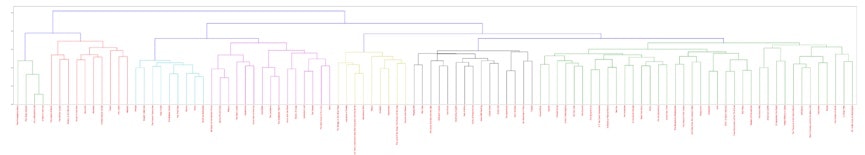
The words are too tiny here. Check out the repository to see more.
Now, we can figure out what could be the best options to recommend to an audience based on their liked movies.