サポートベクトル編
ここではscikit-learn 予測モデルを汎化して現場でコピペTIPS集として掲載します。
条件
1.データ、特徴量
・某エンターテインメント系銘柄の2019年一年分の株価データを使用
・同期間の日経平均インバース・インデックスを使用
・特徴量の最適な組合せか否かバリデーション手法については言及しない
2.モデル
・実装方法を趣旨とし学習不足や過学習、予測値の精度といった評価指標についてパラメータチューニングまで追求しない
サポートベクトル回帰
1.線形回帰
出来高と株価の相関をみる
・回帰線とSVR境界線の傾きを確認する
・マージン内の分布を確認する
・線形回帰とSVR回帰の平均二乗誤差を確認する
import matplotlib.pyplot as plt
import numpy as np
from sklearn.linear_model import LinearRegression
from sklearn.svm import SVR
from sklearn.preprocessing import StandardScaler
from sklearn.model_selection import train_test_split
from sklearn.metrics import mean_squared_error

npArray = np.loadtxt("stock.csv", delimiter = ",", dtype = "float",skiprows=1)

# 特徴量(出来高)
x = npArray[:,2:3]

# 予測データ(株価)
y = npArray[:, 3:4].ravel()

# 訓練データと評価データに分割
x_train, x_test, y_train, y_test = train_test_split(x, y, test_size=0.2)#, random_state=0)

# 特徴量の標準化
sc = StandardScaler()

# 訓練データを変換器で標準化
x_train_std = sc.fit_transform(x_train)
# 訓練データで訓練した変換器でテストデータを標準化
x_test_std = sc.transform(x_test)

# 線形回帰モデルを作成
mod = LinearRegression()
# SVRモデルを作成
mod2 = SVR(kernel='linear', C=10000.0, epsilon=250.0)

# 線形回帰モデル学習
mod.fit(x_train_std, y_train)
# SVR
mod2.fit(x_train_std, y_train)

# 訓練データ(出来高)のプロット
plt.figure(figsize=(8,5))
# 出来高のソート(最小値、最大値間まで0.1刻ndarray作成)
x_ndar = np.arange(x_train_std.min(), x_train_std.max(), 0.1)[:, np.newaxis]

# 出来高の線形回帰予測
y_ndar_prd = mod.predict(x_ndar)
# 出来高のSVR予測
y_ndar_svr = mod2.predict(x_ndar)

## MSE(平均二乗誤差)
mse_train_lin=mod.predict(x_train_std)
mse_test_lin=mod.predict(x_test_std)
mse_train_svr= mod2.predict(x_train_std)
mse_test_svr  = mod2.predict(x_test_std)
# 線形回帰のMSE
print('線形回帰MSE 訓練 = %.1f,テスト = %.1f' % (mean_squared_error(y_train,mse_train_lin),mean_squared_error(y_test, mse_test_lin)))
# SVRのMSE
print('SVRMSE 訓練 = %.1f,テスト =  %.1f' % (mean_squared_error(y_train,mse_train_svr),mean_squared_error(y_test, mse_test_svr)))
random_stateを指定せず数回トライするといずれも当然の事ながらSVRのMSEが少ない
1回目
線形回帰のMSE 訓練 = 38153.4 ,テスト = 33161.9
SVRのMSE 訓練 = 52439.9 ,テスト = 56707.7
2回目
線形回帰のMSE 訓練 = 37836.4 ,テスト = 33841.3
SVRのMSE 訓練 = 54044.5 ,テスト = 51083.7
3回目
線形回帰のMSE 訓練 = 37381.3 ,テスト = 35616.6
SVRのMSE 訓練 = 53499.2 ,テスト = 53619.4
以下でこれを散布図にプロットしてみよう
# 出来高と株価の散布図
plt.scatter(x_train_std, y_train, color='blue', label='data')
# 回帰直線
plt.plot(x_ndar, y_ndar_prd, color='green', linestyle='-', label='LinearRegression')
# 境界線
plt.plot(x_ndar, y_ndar_svr ,color='red', linestyle='-', label='SVR')
# マージン線
plt.plot(x_ndar, y_ndar_svr + mod2.epsilon, color='orange', linestyle='-.', label='margin')
plt.plot(x_ndar, y_ndar_svr - mod2.epsilon, color='orange', linestyle='-.')
# ラベル
plt.ylabel('Closing price')
plt.xlabel('Volume')
plt.title('SVR Regression')
# 凡例
plt.legend(loc='lower right')

plt.show()
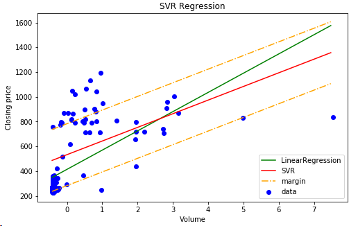
回帰線の傾きよりSVRの境界線のほうがなだらかとなる
マージンをepsilonを250円でとってみたが出来高に合わせ株価も目立った投げもなく概ね順調に上昇基調で推移しているといって良さそうだ。