回帰分析編
ここではscikit-learnの予測モデルを汎化して現場でコピペTIPS集として掲載します。
条件
1.データ、特徴量
・某エンターテインメント系銘柄の2019年一年分の株価データを使用
・同期間の日経平均インバース・インデックスを使用
・特徴量の最適な組合せか否かバリデーション手法については言及しない
2.モデル
・実装方法を趣旨とし学習不足や過学習、予測値の精度といった評価指標についてパラメータチューニングまで追求しない
線形回帰
1.単回帰
インバース・インデックスと株価の相関をみる
import matplotlib.pyplot as plt
import numpy as np
from sklearn.linear_model import LinearRegression
npArray = np.loadtxt("stock.csv", delimiter = ",", dtype = "float",skiprows=1)

# 特徴量(インバースインデックス)
z = npArray[:,1:2]
z = npArray[:,2:3]
# 予測データ(株価)
y = npArray[:, 3:4].ravel()

# 単回帰モデル作成
model = LinearRegression()

# 訓練
model.fit(z,y)
print('傾き:', model.coef_)
print('切片:', model.intercept_)

# 予測
y_pred = model.predict(z)

# INDEXと株価の散布図と1次関数のプロット
plt.figure(figsize=(8,4))
plt.scatter(z,y, color='blue', label='Stock price')
plt.plot(z,y_pred, color='green', linestyle='-', label='LinearRegression')

# 出来高プロット
plt.ylabel('Closing price')
plt.xlabel('Volume')
plt.title('Regression Analysis')
plt.legend(loc='lower right')
傾き: [-2.27391593]
切片: 4795.89427740762
インバースインデックスと株価は負の相関となり連動していない事が判る

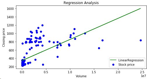
では次に出来高と株価の相関を見てみよう
今度は正の相関となり一年を通してほぼ安定した上昇基調であった事が読み取れる。
2.重回帰
インバース・インデックスと出来高から株価のMSE(平均二乗誤差)と予測株価の残差をみる
import matplotlib.pyplot as plt
import numpy as np
from sklearn.linear_model import LinearRegression
from sklearn.preprocessing import StandardScaler
from sklearn.model_selection import train_test_split
from sklearn.metrics import mean_squared_error
npArray = np.loadtxt("stock.csv", delimiter = ",", dtype = "float",skiprows=1)
# 特徴量(インバース・インデックス&出来高)
x = npArray[:,1:3]
# 予測データ(株価)
y = npArray[:, 3:4].ravel()
# 重回帰モデル作成
model = LinearRegression()
# 特徴量標準化
sc = StandardScaler()

# 訓練データ(INDEX,出来高)の標準化の変換機を訓練
x_train_std = sc.fit_transform(x_train)
# 訓練データで訓練した変換器でテストデータ(INDEX,出来高)を標準化する
x_test_std = sc.transform(x_test)

# 訓練データでモデルの学習
model.fit(x_train_std, y_train)

# 訓練データ、テストデータで株価を予測
y_train_prd = model.predict(x_train_std)
y_test_prd = model.predict(x_test_std)

# 実株価と予測株価のMSEを計算
np.mean((y_train - y_train_prd) ** 2)
np.mean((y_test - y_test_prd) ** 2)

# MSE(平均二乗誤差)の計算
print('MSE ', mean_squared_error(y_train, y_train_prd),mean_squared_error(y_test, y_test_prd))

# 予測株価残差(予測-正解)のプロット
plt.figure(figsize=(7,5))
plt.scatter(y_train_prd,  y_train_prd - y_train,
c='orange', marker='s', edgecolor='white',
label='Training')
plt.scatter(y_test_prd,  y_test_prd - y_test,
c='blue', marker='s', edgecolor='white',
label='Test')

plt.xlabel('Stock price')
plt.ylabel('Residual error')
plt.legend(loc='upper left')
plt.hlines(y=0, xmin=0, xmax=1200, color='green', ls='dashed',lw=2)
plt.xlim([220,1200])
plt.tight_layout()
plt.show()
最小二乗平均は 訓練データ = 17349.4,テストデータ 23046.2
上記の様にインバースインデックスと株価は負の相関関係だった事もありMSEの値は高く訓練データとの差も大きい

株価が300円前後の2019前半は比較的残差は少ないもののインバースインデックスとは負の相関を見せている事もあり500円を超えた頃からはバラつきが大きく訓練データとの誤差も大きい事から株価の予測にはなりえない事が判る
続く