はじめに
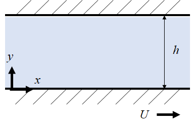
下図の様に距離$h$離れた2枚の平行平板間が流体で満たされている状態を考える。下の板は静止し上の板がある速度$U$で$x$方向に動いているとき平板間に発生する流れを一般的にクエット流(Couette flow)と呼ぶ。
平板間の流体が非圧縮性粘性流体であると仮定したとき、質量保存則及び運動量保存則より、流れの運動方程式は以下の様に記述できる。
$$
\begin{equation}
\frac{\partial u}{\partial t} = \nu \frac{\partial^2 u}{\partial y^2} \tag{1}
\end{equation}
$$
ここで$\nu$は流体の動粘性係数、$u$は$x$方向の速度成分である。
時間$t=0$の時、両平板及び流体は静止しているものとし、$t>0$において上の平板が速度$U$で動き始めるとき、境界条件は下記の通りに表される。
$$
{\displaystyle u(y,0)=0,\quad 0<y<h,} \tag{2}
$$
$$
{\displaystyle u(0,t)=0,\quad u(h,t)=U,\quad t>0.} \tag{3}
$$
この時、運動方程式(1)は解析的に解くことができる。解析解は以下の様に表される。
{\displaystyle u(y,t)=U{\frac {y}{h}}-{\frac {2U}{\pi }}\sum _{n=1}^{\infty }{\frac {1}{n}}e^{-n^{2}\pi ^{2}\nu t/h^{2}}\sin \left[n\pi \left(1-{\frac {y}{h}}\right)\right]} \tag{4}
解析解の導出に関しては参考文献1を参照されたい。
参考文献1:D. J. Acheson, Elementary fluid dynamics, Oxford University Press, (1990)
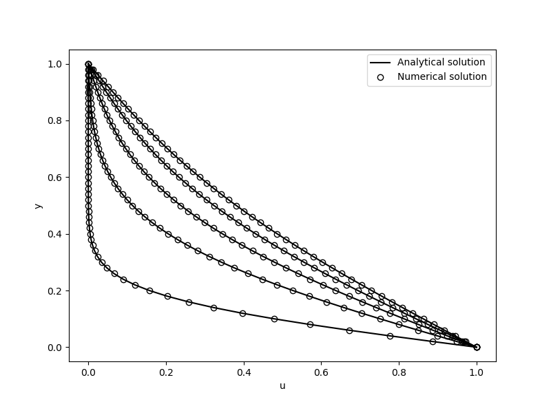
Pythonによるシミュレーション
上記運動方程式(1)を数値的に解き、解析解との比較を行う。式(1)の右辺の粘性項は2次精度の中心差分を用いて離散化した。また時間積分には2次精度のRunge-Kutta法を用いた。
import numpy as np
import matplotlib.pyplot as plt

''' Analytical solution of Couette flow '''
def u_exact(U,h,nu,y,t):
    u = U * (1-y / h)
    for n in range(1,100000):
        u -= 2 * U / np.pi * (1/n) *  np.e **(-n**2*np.pi**2*nu*t/h**2)*np.sin(n*np.pi*y/h)
    return u

''' Parameters '''
h = 1   # gap between plate
U = 1   # velocity of under wall
nu = 0.0005 # viscosity coefficient

nx = 51 # number of mesh

y = h * np.linspace(0,1,nx) # y coordinates
dy = h / (nx-1) # mesh size
dt = 0.02   # timestep
nend = 20000    # number of iteration

''' Initial conditions '''
u = np.zeros(nx)
un = np.zeros(nx)
u1 = np.zeros(nx)

u[0] = U
u1[0] = U
un[0] = U

''' 2nd order Runge-Kutta '''
for nt in range(nend):
    u1[1:nx-1] = u[1:nx-1] + 0.5 * dt * nu * (u[0:nx-2] - 2 * u[1:nx-1] + u[2:nx]) / dy**2

#    for j in range(1,nx-1):
#        u1[j] = u[j] + 0.5* dt * nu * (u[j-1] - 2 * u[j] + u[j+1]) / dy**2

    un[1:nx-1] = u[1:nx-1] + dt * nu * (u1[0:nx-2] - 2 * u1[1:nx-1] + u1[2:nx]) / dy**2
#    for j in range(1,nx-1):
#        un[j] = u[j] + dt * nu * (u1[j-1] - 2 * u1[j] + u1[j+1]) / dy**2

    u = un.copy()

    ''' Plot '''
    if np.mod(nt + 3000, 4000) == 0 and nt < 5000 and nt > 0:
        ue = u_exact(U,h,nu,y,dt*nt)

        plt.plot(ue,y, color = 'black', label = "Analytical solution")
        plt.plot(un,y,"o", color = 'None', markeredgecolor='black', label = "Numerical solution")


    elif np.mod(nt + 3000, 4000) == 0 and nt > 0:
        ue = u_exact(U,h,nu,y,dt*nt)

        plt.plot(ue,y, color = 'black')
        plt.plot(un,y,"o", color = 'None', markeredgecolor='black')

plt.xlabel("u")
plt.ylabel("y")
plt.legend()
plt.show()