はじめに
OpenModelica(以下、OM)はパラメータスタディ機能や結果の処理、分析、可視化機能が弱く物足りないことがある。
OMにはPythonとの連携機能があるので、計算の実行や結果の処理をPythonで行うことでOMに足りない部分を補うことができるかもしれない。
それを確認するためまずPython-OM連携機能の動作検証を行いPandasというデータ分析ライブラリで計算結果の処理を行ってみる。
Pythonはほぼ未経験者のため間違いがあればご指摘ください。
OM-Python連携機能
OMにはPythonとの連携機能が3つある。
主にPythonからOMのコマンドを実行するものである。
- OMPython
OpenModelicaShell(以下、OMShell)のコマンドをそのままPythonから実行するツール
Pthonからシミュレーションを実行するコマンド
OMShellでシミュレーションを実行するには 'simulate(~~)' となるので
sendExpressionでそのままコードを渡していることが分かる
omc.sendExpression("simulate(BouncingBall, stopTime=3.0)")
- EnhancedOMPython
OMShellのコマンドではなく、より簡便なコマンドでOMを操作できるツール
以下はOMPythonと同様にシミュレーションを実行するコマンド
短く簡潔になっていることが分かる
mod.simulate()
- PySimulator
グラフィカルにModelicaモデルやFMUモデルを実行し結果表示できるツール
詳しくは以下参照
https://github.com/PySimulator/PySimulator
OMPythonの動作検証
一番ベーシックなOMPythonについて動作検証を行う。
Python側の実行はJupyterLabで行う。
環境
Windows10 Home 1809
conda version : 4.5.4
conda-build version : 3.10.5
python version : 3.6.5.final.0
JupyterLab : 1.2.6
OpenModelica : 1.13.2 64bit
インストール
以下のReadMeに従ってインストールする。
https://github.com/OpenModelica/OMPython
事前にOM, Anacondaをインストールしていることが前提となる。
①. Anaconda Promptを起動し、以下のフォルダに移動
ここで「%OPENMODELICAHOME%」はOMがインストールされているフォルダ直下のパス
cd %OPENMODELICAHOME%\share\omc\scripts\PythonInterface
②. 以下のコマンドでインストール
python -m pip install -U .
こんなメッセージが出てきた。
Could not install packages due to an EnvironmentError: [WinError 5] アクセスが拒否されました。: 'C:\\Program Files (x86)\\Microsoft Visual Studio\\Shared\\Anaconda3_64\\Lib\\site-packages\\future'
Consider using the `--user` option or check the permissions.
エラーメッセージがすごい親切。言われたとおり--userをつけて再実行。出来た。
python -m pip install --user -U .
メッセージ
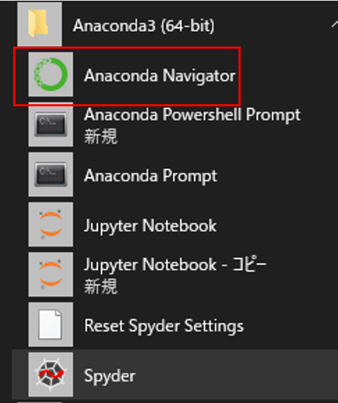
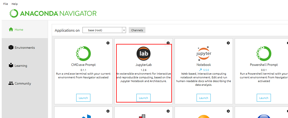
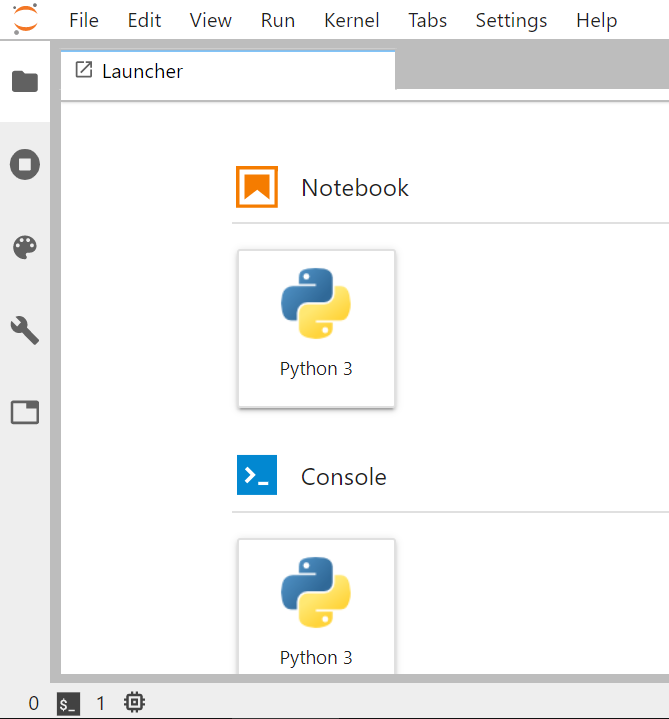
③. インストールされたかどうか確認するためJupyterLabを起動する。起動方法はAnaconda Navigatorをスタートメニューから起動して「JupyterLab」を起動。NotebookのPythonを選択する。
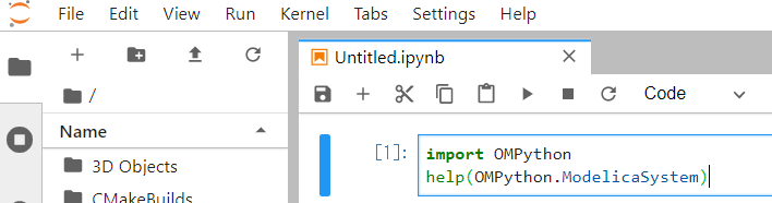
④. 以下を実行
import OMPython
help(OMPython.ModelicaSystem)
JupyterLabの画像だとこんな感じ。直感的で操作しやすい。
Ctrl + エンターで実行。セルの挿入はb、削除はdを2回。
以下の結果が返ってきたら成功
Help on class ModelicaSystem in module OMPython:
class ModelicaSystem(builtins.object)
| Methods defined here:
|
| del(self)
|
| init(self, fileName=None, modelName=None, lmodel=[], useCorba=False)
| "constructor"
| It initializes to load file and build a model, generating object, exe, xml, mat, and json files. etc. It can be called :
| •without any arguments: In this case it neither loads a file nor build a model. This is useful when a FMU needed to convert to Modelica model
| •with two arguments as file name with ".mo" extension and the model name respectively
| •with three arguments, the first and second are file name and model name respectively and the third arguments is Modelica standard library to load a model, which is common in such models where the model is based on the standard library. For example, here is a model named "dcmotor.mo" below table 4-2, which is located in the directory of OpenModelica at "C:\OpenModelica1.9.4-dev.beta2\share\doc\omc estmodels".
| Note: If the model file is not in the current working directory, then the path where file is located must be included together with file name. Besides, if the Modelica model contains several different models within the same package, then in order to build the specific model, in second argument, user must put the package name with dot(.) followed by specific model name.
| ex: myModel = ModelicaSystem("ModelicaModel.mo", "modelName")
|
| convertFmu2Mo(self, fmuName)
| In order to load FMU, at first it needs to be translated into Modelica model. This method is used to generate Modelica model from the given FMU. It generates "fmuName_me_FMU.mo". It can be called:
| •only without any arguments
| Currently, it only supports Model Exchange conversion.
|
| - Input arguments: s1
| * s1: name of FMU file, including extension .fmu
|
| convertMo2Fmu(self)
| This method is used to generate FMU from the given Modelica model. It creates "modelName.fmu" in the current working directory. It can be called:
| •only without any arguments
|
| getContinuous(self, *names)
| This method returns dict. The key is continuous names and value is corresponding continuous value.
| If *name is None then the function will return dict which contain all continuous names as key and value as corresponding values. eg., getContinuous()
| Otherwise variable number of arguments can be passed as continuous name in string format separated by commas. eg., getContinuous('cName1', 'cName2')
|
| getInputs(self, *names)
| This method returns dict. The key is input names and value is corresponding input value.
| If *name is None then the function will return dict which contain all input names as key and value as corresponding values. eg., getInputs()
| Otherwise variable number of arguments can be passed as input name in string format separated by commas. eg., getInputs('iName1', 'iName2')
|
| getLinearInputs(self)
|
| getLinearOutputs(self)
|
| getLinearQuantityInformation(self)
|
| getLinearStates(self)
|
| getLinearizationOptions(self, *names)
| This method returns dict. The key is linearize option names and value is corresponding linearize option value.
| If *name is None then the function will return dict which contain all linearize option names as key and value as corresponding values. eg., getLinearizationOptions()
| Otherwise variable number of arguments can be passed as simulation option name in string format separated by commas. eg., getLinearizationOptions('linName1', 'linName2')
|
| getOptimizationOptions(self, *names)
|
| getOutputs(self, *names)
| This method returns dict. The key is output names and value is corresponding output value.
| If *name is None then the function will return dict which contain all output names as key and value as corresponding values. eg., getOutputs()
| Otherwise variable number of arguments can be passed as output name in string format separated by commas. eg., getOutputs(opName1', 'opName2')
|
| getParameters(self, *names)
| This method returns dict. The key is parameter names and value is corresponding parameter value.
| If *name is None then the function will return dict which contain all parameter names as key and value as corresponding values. eg., getParameters()
| Otherwise variable number of arguments can be passed as parameter name in string format separated by commas. eg., getParameters('paraName1', 'paraName2')
|
| getQuantities(self, names=None)
| This method returns list of dictionaries. It displays details of quantities such as name, value, changeable, and description, where changeable means if value for corresponding quantity name is changeable or not. It can be called :
| •without argument: it returns list of dictionaries of all quantities
| •with a single argument as list of quantities name in string format: it returns list of dictionaries of only particular quantities name
| •a single argument as a single quantity name (or in list) in string format: it returns list of dictionaries of the particular quantity name
|
| getSimulationOptions(self, *names)
| This method returns dict. The key is simulation option names and value is corresponding simulation option value.
| If *name is None then the function will return dict which contain all simulation option names as key and value as corresponding values. eg., getSimulationOptions()
| Otherwise variable number of arguments can be passed as simulation option name in string format separated by commas. eg., getSimulationOptions('simName1', 'simName2')
|
| getSolutions(self, *varList)
| This method returns tuple of numpy arrays. It can be called:
| •with a list of quantities name in string format as argument: it returns the simulation results of the corresponding names in the same order. Here it supports Python unpacking depending upon the number of variables assigned.
|
| linearize(self)
| This method linearizes model according to the linearized options. This will generate a linear model that consists of matrices A, B, C and D. It can be called:
| •only without any arguments
|
| optimize(self)
| This method optimizes model according to the optimized options. It can be called:
| •only without any arguments
|
| requestApi(self, apiName, entity=None, properties=None)
| # request to OMC
|
| setContinuous(self, **cvals)
| This method is used to set continuous values. It can be called:
| •with a sequence of continuous name and assigning corresponding values as arguments as show in the example below:
| setContinuousValues(cName1 = 10.9, cName2 = 0.066)
|
| setInputs(self, **nameVal)
| This method is used to set input values. It can be called:
| •with a sequence of input name and assigning corresponding values as arguments as show in the example below:
| setParameterValues(iName = [(t0, v0), (t1, v0), (t1, v2), (t3, v2)...]), where tj<=tj+1
|
| setLinearizationOptions(self, **linearizationOptions)
| This method is used to set linearization options. It can be called:
| •with a sequence of linearization options name and assigning corresponding value as arguments as show in the example below
| setLinearizationOptions(stopTime=0, stepSize = 10)
|
| setOptimizationOptions(self, **optimizationOptions)
| This method is used to set optimization options. It can be called:
| •with a sequence of optimization options name and assigning corresponding values as arguments as show in the example below:
| setOptimizationOptions(stopTime = 10,simflags = '-lv LOG_IPOPT -optimizerNP 1')
|
| setParameters(self, **pvals)
| This method is used to set parameter values. It can be called:
| •with a sequence of parameter name and assigning corresponding value as arguments as show in the example below:
| setParameterValues(pName1 = 10.9, pName2 = 0.066)
|
| setSimulationOptions(self, **simOptions)
| This method is used to set simulation options. It can be called:
| •with a sequence of simulation options name and assigning corresponding values as arguments as show in the example below:
| setSimulationOptions(stopTime = 100, solver = 'euler')
|
| simulate(self)
| This method simulates model according to the simulation options. It can be called:
| •only without any arguments: simulate the model
|
| ----------------------------------------------------------------------
| Data descriptors defined here:
|
| dict
| dictionary for instance variables (if defined)
|
| weakref
| list of weak references to the object (if defined)
テストモデルの実行
以下の公式チュートリアルに従って実行する。
計算対象はバウンドするボールの挙動。
https://www.openmodelica.org/doc/OpenModelicaUsersGuide/OpenModelicaUsersGuide-v1.13.2.pdf
①. 計算実行のためモデルの読み込みやフォルダの移動など実行
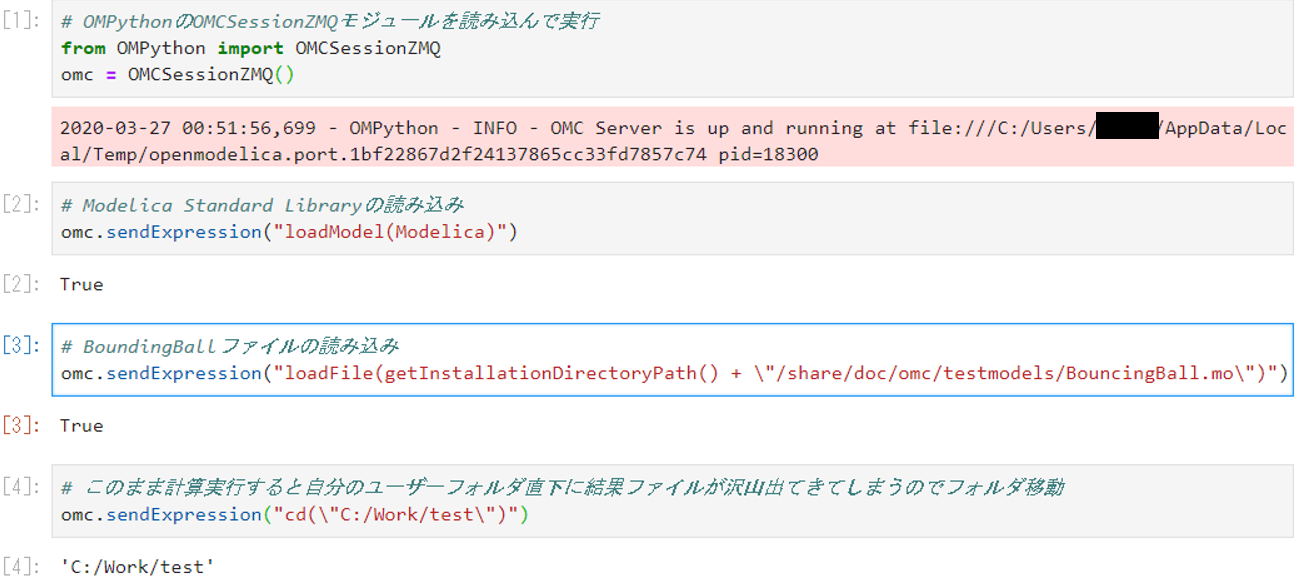
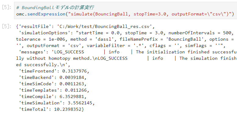
②.計算の実行
後ほどPandasで結果処理をするためcsvで出力
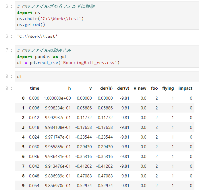
③. 計算値の取得
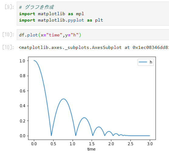
④. 結果のプロット
所感
Python, JupyterLabは直感的で操作しやすい。
Pandasも慣れれば多分大丈夫。
簡単な操作性でデータ分析の標準的なツールということなのも納得がいった。
ただ、結果の確認や処理がコマンドベースなのでMATLABやExcelのように
もっとグラフィカルにマウスでデータを選択してボタンをポチポチしていくだけでグラフを作れたら嬉しい。
計算実行、データの加工(必要な結果の抜き出し、平均化や差分)などの処理はPython、
処理された数値に対してグラフ作成や提出用のレポート作成はExcelなど使い分けてもいいと思う。
追記
以下の記事でExcelとPythonの使い分けについて大変分かりやすい考察があった。
https://qiita.com/taka000826/items/ca8fa4a1a392728f688c
OMPythonは問題なく動作するし、十分役割を果たしてくれた。
結局OMShellのコマンドをそのままたたいているだけだが
OMShellで苦手な動作をPythonがカバーしてくれるので大変助かる。
今後も使っていこうと思う。