Yahoo Financeのデータ（S&P500）を使って、DDQNにトレーディングを学習させてみた

はじめに

今回は、「ChatGPTにハンズオンを作らせてみた」の第10弾で、DDQN（Double Deep Q Network）を用いて、S&P500のデータを使ってアルゴリズムトレーディングを実装しました。

第9弾はこちら↓

DDQN（Double Deep Q Network）

Q値の更新を「次の行動を選択するためのネットワーク（現在のネットワーク）」と「その行動のQ値を評価するためのネットワーク（ターゲットネットワーク）」の2つを用いることで、DQNの価値を過大評価してしまう欠点を防ぐために改良された手法。

使用コード・分析結果

import numpy as np
import pandas as pd
import yfinance as yf
import gym
import matplotlib.pyplot as plt
from collections import deque
import random

import tensorflow as tf
from tensorflow.keras.models import Sequential
from tensorflow.keras.layers import Dense
from tensorflow.keras.optimizers import Adam

Yahoo FinanceからS&P500の価格データ（終値）を取得します。2018年から2022年までの期間を学習データ、2023年を検証データとして分割します。また、終値に加えて、10日移動平均（SMA_10）と50日移動平均（SMA_50）も変数として追加しています。

import yfinance as yf
import pandas as pd

# 取得する銘柄
ticker = "SPY"

# 期間設定（2024年1月1日まで）
start_date = "2018-01-01"
end_date = "2024-01-01"

# データ取得
data = yf.download(ticker, start=start_date, end=end_date)

# 必要なカラムのみ
data = data[['Close']]

# 移動平均線（SMA）の特徴量を追加
data['SMA_10'] = data['Close'].rolling(window=10).mean()
data['SMA_50'] = data['Close'].rolling(window=50).mean()

# NaNがある行を削除（移動平均の計算後）
data.dropna(inplace=True)

# インデックスを日付に設定
data.index = pd.to_datetime(data.index)

# データを分割
train_data = data[:'2022-12-31']  # 2022年までを学習データ
test_data = data['2023-01-01':]  # 2023年を検証データ

# データの確認
print("学習データ (Train) の範囲:", train_data.index.min(), "〜", train_data.index.max())
print("検証データ (Test) の範囲:", test_data.index.min(), "〜", test_data.index.max())

取引環境を作成し、DDQNエージェントが学習できるようにします。

import gym
import numpy as np
import pandas as pd

class StockTradingEnv(gym.Env):
    def __init__(self, df):
        super(StockTradingEnv, self).__init__()

        self.df = df.reset_index()
        self.current_step = 0
        self.cash = 10000  # 初期資金
        self.shares_held = 0  # 持ち株数
        self.total_reward = 0  # 累積リワード
        self.history = []  # 資産履歴を保存するリスト

        self.action_space = gym.spaces.Discrete(3)
        self.observation_space = gym.spaces.Box(
            low=0, high=np.inf, shape=(3,), dtype=np.float32
        )

    def reset(self):
        self.current_step = 0
        self.cash = 10000
        self.shares_held = 0
        self.total_reward = 0
        self.history = []  # 履歴をリセット
        return self._next_observation()

    def _next_observation(self):
        obs = np.array([
            float(self.df.iloc[self.current_step]['Close']),
            float(self.df.iloc[self.current_step]['SMA_10']),
            float(self.df.iloc[self.current_step]['SMA_50'])
        ], dtype=np.float32)
        return obs

    def step(self, action):
        current_price = float(self.df.iloc[self.current_step]['Close'])
        self.current_step += 1

        # 売買ロジック
        if action == 1 and self.cash >= current_price:  # 買い
            self.shares_held += 1
            self.cash -= current_price
        elif action == 2 and self.shares_held > 0:  # 売り
            self.shares_held -= 1
            self.cash += current_price

        # 総資産計算
        total_value = self.cash + (self.shares_held * current_price)
        reward = total_value - 10000
        self.total_reward += reward

        # 資産履歴を保存
        self.history.append(total_value)

        done = self.current_step >= len(self.df) - 1
        return self._next_observation(), reward, done, {}

    def get_equity_curve(self):
        """ 累積リターンを取得 """
        return self.history

DDQNエージェントを作成し、学習を行います。

class DDQNAgent:
    def __init__(self, state_size, action_size):
        self.state_size = state_size
        self.action_size = action_size
        self.memory = deque(maxlen=1000)
        self.gamma = 0.95
        self.epsilon = 1.0
        self.epsilon_min = 0.01
        self.epsilon_decay = 0.995
        self.learning_rate = 0.001
        self.model = self._build_model()
        self.target_model = self._build_model()
        self.update_target_model()

    def _build_model(self):
        model = Sequential([
            Dense(24, input_dim=self.state_size, activation="relu"),
            Dense(24, activation="relu"),
            Dense(self.action_size, activation="linear")
        ])
        model.compile(loss="mse", optimizer=Adam(learning_rate=self.learning_rate))
        return model

    def update_target_model(self):
        self.target_model.set_weights(self.model.get_weights())

    def act(self, state):
        if np.random.rand() <= self.epsilon:
            return random.randrange(self.action_size)
        q_values = self.model.predict(state)
        return np.argmax(q_values[0])

    def train(self, batch_size=32):
        minibatch = random.sample(self.memory, batch_size)
        for state, action, reward, next_state, done in minibatch:
            target = reward
            if not done:
                target = reward + self.gamma * np.amax(self.target_model.predict(next_state)[0])
            target_f = self.model.predict(state)
            target_f[0][action] = target
            self.model.fit(state, target_f, epochs=1, verbose=0)
        if self.epsilon > self.epsilon_min:
            self.epsilon *= self.epsilon_decay

上記で定義したエージェントを実際に学習させて、評価します。

agent = DDQNAgent(state_size=3, action_size=3)
episodes = 100

for e in range(episodes):
    state = env.reset().reshape(1, 3)
    done = False
    total_reward = 0

    while not done:
        action = agent.act(state)
        next_state, reward, done, _ = env.step(action)
        next_state = next_state.reshape(1, 3)
        agent.memory.append((state, action, reward, next_state, done))
        state = next_state
        total_reward += reward

    agent.train()
    agent.update_target_model()
    print(f"Episode {e+1}/{episodes}, Total Reward: {total_reward}")

エージェントの学習には時間がかかるので、学習させたモデルを保存しておきます。

# keras 形式で保存
agent.model.save("ddqn_trading_model.keras")

エージェントの資産推移をグラフ化するための関数を定義します。

import matplotlib.pyplot as plt

def plot_equity_curve(env):
    equity_curve = env.get_equity_curve()

    plt.figure(figsize=(10, 5))
    plt.plot(equity_curve, label="Total Asset ($)")
    plt.axhline(y=10000, color='r', linestyle='--', label="Initial Capital ($10,000)")
    plt.xlabel("Time Steps")
    plt.ylabel("Total Asset ($)")
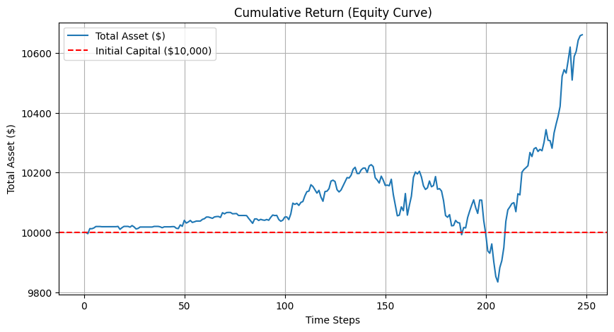
    plt.title("Cumulative Return (Equity Curve)")
    plt.legend()
    plt.grid()
    plt.show()

学習済みモデルを読み込み、検証用データ（2023年）で検証していきます。

# 1. 学習後のモデルを保存（.keras 形式）
agent.model.save("ddqn_trading_model.keras")

# 2. 検証データを使った評価
from tensorflow.keras.models import load_model

# 学習済みモデルをロード
trained_model = load_model("ddqn_trading_model.keras")

# 検証用のエージェント（同じネットワーク構造）
test_agent = DDQNAgent(state_size=3, action_size=3)
test_agent.model = trained_model  # モデルを置き換え

# 検証用の環境を作成
test_env = StockTradingEnv(test_data)

# 検証開始
state = test_env.reset().reshape(1, 3)
done = False

while not done:
    action = test_agent.act(state)  # エージェントの予測
    next_state, _, done, _ = test_env.step(action)
    state = next_state.reshape(1, 3)

# 検証後に累積リターンをプロット
plot_equity_curve(test_env)

元の価格の推移も可視化しておきます。

plt.figure(figsize=(10, 5))
plt.plot(test_data['Close'], label="Close Price")

検証データでのパフォーマンスを定量的に評価するために、各指標を計算します。

import numpy as np

# 累積リターンの取得
equity_curve = np.array(test_env.get_equity_curve())

# ① リターンの計算
returns = np.diff(equity_curve) / equity_curve[:-1]  # 日次リターン

# ② 平均リターン
mean_return = np.mean(returns)

# ③ 標準偏差（リスク）
std_return = np.std(returns)

# ④ シャープレシオ（リスク調整後のリターン）
risk_free_rate = 0.02 / 252  # 年率2%を1日あたりに換算
sharpe_ratio = (mean_return - risk_free_rate) / std_return

# ⑤ 最大ドローダウン
cumulative_returns = (equity_curve - 10000) / 10000  # 累積リターン
peak = np.maximum.accumulate(cumulative_returns)
drawdown = (peak - cumulative_returns)
max_drawdown = np.max(drawdown)

# ⑥ 勝率（トレードの成功率）
winning_trades = np.sum(returns > 0)
total_trades = len(returns)
win_rate = winning_trades / total_trades

# 結果を表示
print(f"✅ 平均リターン: {mean_return:.5f}")
print(f"✅ 標準偏差（リスク）: {std_return:.5f}")
print(f"✅ シャープレシオ: {sharpe_ratio:.2f}")
print(f"✅ 最大ドローダウン: {max_drawdown:.2f}")
print(f"✅ 勝率: {win_rate:.2%}")

✅ 平均リターン: 0.00026
✅ 標準偏差（リスク）: 0.00235
✅ シャープレシオ: 0.08
✅ 最大ドローダウン: 0.04
✅ 勝率: 50.40%

考察

一つ目のグラフを見てみると、最終的にはそれなりに利益が出ているように見えますが、元の価格推移と比較すると、めちゃくちゃ相関しているように見えます。

各指標を見てみても、

• 平均リターンが低い：利益は出ているが、小さい
• 標準偏差が低い：リスクが低い
• シャープレシオが低い：リスクに見合ったリターンが得られていない
• 最大ドローダウンが約4%：許容範囲内だが、改善の余地がある
• 勝率が約50%：ほぼランダム

という結果になり、まだ学習が足りていないような気がしますね。

おわりに

まだまだ改善の余地がありそうなので、もう少し改善してみようと思います