はじめに
今回は、「ChatGPTにハンズオンを作らせてみた」の第4弾で、傾向スコアマッチングを勉強しました。
第3弾はこちら↓
傾向スコアマッチング
因果推論の手法の一つで、「似たような条件のデータ同士」をペアにすることで、2つのグループをできるだけ公平に比べることができます。
使用データ
Kaggleのデータセットである、「Medical Cost Personal Datasets」という個人の医療費に関するデータを含むデータセットを用いました。その中でも、今回は次の6つの変数をピックアップして使用しました。
| 変数 | 説明 |
|---|---|
| age | 年齢 |
| sex | 性別 |
| bmi | BMI |
| children | 子どもの数 |
| smoker | 喫煙者かどうか |
| charges | 医療費 |
また、このデータを用いて、次の変数を作成しました。
| 変数 | 説明 |
|---|---|
| propensity_score | 傾向スコア(喫煙者である確率) |
やること
上記のデータを用いて、喫煙者・非喫煙者の違いによって、医療費に違いが出るかを傾向スコアマッチングを用いて確かめます。具体的な手順は次の通りです。
- ロジスティック回帰で傾向スコアを算出
- 1対1で最近傍マッチング
- マッチング前後の平均値の違いを比較
使用コード
import numpy as np
import pandas as pd
import matplotlib.pyplot as plt
import seaborn as sns
from sklearn.linear_model import LogisticRegression
from sklearn.preprocessing import StandardScaler
from sklearn.metrics import roc_auc_score
from scipy.spatial import distance
from statsmodels.stats.weightstats import ttest_ind
ダウンロードしたデータを取得したうえで、smokerがyes, noの二値を取っているので、それぞれ1, 0に変換します。
df = pd.read_csv("data/insurance.csv")
df['smoker'] = df['smoker'].map({'yes': 1, 'no': 0})
age, sex, bmi, childrenを説明変数、smorkerを目的変数として、ロジスティック回帰で「喫煙者である確率」を算出し、propensity_scoreとして格納します。
# 説明変数(共変量)を選択(年齢, 性別, BMI, 子供の数)
X = df[['age', 'sex', 'bmi', 'children']]
y = df['smoker']
# 標準化
scaler = StandardScaler()
X_scaled = scaler.fit_transform(X)
# ロジスティック回帰で傾向スコア推定
logit = LogisticRegression()
logit.fit(X_scaled, y)
# 傾向スコアの取得
df['propensity_score'] = logit.predict_proba(X_scaled)[:, 1]
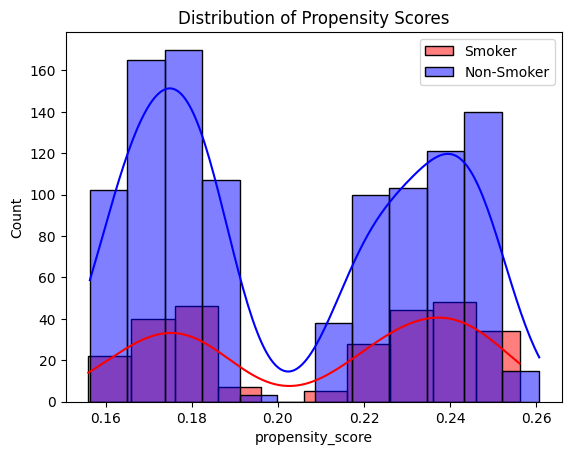
# 傾向スコアの分布を確認
sns.histplot(df[df['smoker'] == 1]['propensity_score'], color='red', alpha=0.5, label='Smoker', kde=True)
sns.histplot(df[df['smoker'] == 0]['propensity_score'], color='blue', alpha=0.5, label='Non-Smoker', kde=True)
plt.legend()
plt.title("Distribution of Propensity Scores")
plt.show()
傾向スコアが喫煙者・非喫煙者ともに似たような分布をしており、あまり明確に分離できていない可能性がある。別の手法で傾向スコアを算出することもできるが、今回は一旦そのまま進みます。
傾向スコアをもとに、各喫煙者と最も似ている非喫煙者1人を最近傍法を用いてマッチングします。
from scipy.spatial import distance
# 傾向スコアを float 型に変換
df['propensity_score'] = df['propensity_score'].astype(float)
# 処置群と対照群のデータ
treated = df[df['smoker'] == 1].copy()
control = df[df['smoker'] == 0].copy()
# 最近傍マッチング
matched_indices = []
for i, row in treated.iterrows():
# 適切な形式に変換
treated_score = np.array([[row['propensity_score']]]) # 2D array にする
control_scores = control[['propensity_score']].to_numpy() # 2D array にする
# 最近傍マッチングのインデックスを取得
min_idx = distance.cdist(treated_score, control_scores).argmin()
# インデックスをリストに追加
matched_indices.append(control.index[min_idx])
# マッチング後のデータ
matched_control = df.loc[matched_indices].copy()
matched_treated = treated.copy()
# マッチング後のデータセット作成
matched_df = pd.concat([matched_treated, matched_control])
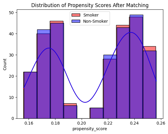
# マッチング後の傾向スコア分布確認
sns.histplot(matched_df[matched_df['smoker'] == 1]['propensity_score'], color='red', alpha=0.5, label='Smoker', kde=True)
sns.histplot(matched_df[matched_df['smoker'] == 0]['propensity_score'], color='blue', alpha=0.5, label='Non-Smoker', kde=True)
plt.legend()
plt.title("Distribution of Propensity Scores After Matching")
plt.show()
マッチング前と比較して、喫煙者と非喫煙者の分布がほぼ一致しており、適切にマッチングできたと考えられる。
マッチング前後で、喫煙者・非喫煙者の間で各説明変数のバランスが崩れていないかを確認するため、平均値を確認しておきます。
# マッチング前後の共変量の平均比較
before_matching = df.groupby('smoker')[['age', 'bmi', 'children']].mean()
after_matching = matched_df.groupby('smoker')[['age', 'bmi', 'children']].mean()

balance_check = pd.concat([before_matching, after_matching], keys=['Before Matching', 'After Matching'])

from IPython.display import display

display(balance_check)
| Matching Stage | Smoker | Age | BMI | Children |
|---|---|---|---|---|
| Before Matching | 0 (Non-Smoker) | 39.39 | 30.65 | 1.09 |
| 1 (Smoker) | 38.51 | 30.71 | 1.11 | |
| After Matching | 0 (Non-Smoker) | 38.43 | 31.51 | 1.03 |
| 1 (Smoker) | 38.51 | 30.71 | 1.11 |
マッチングの効果の確認
1. 年齢 (age)
-
マッチング前
- 非喫煙者: 39.39
- 喫煙者: 38.51
- → 1歳弱の差があった
-
マッチング後
- 非喫煙者: 38.43
- 喫煙者: 38.51
- → 差が縮まり、バランスが改善
2. BMI (bmi)
-
マッチング前
- 非喫煙者: 30.65
- 喫煙者: 30.71
- → ほぼ差はなし
-
マッチング後
- 非喫煙者: 31.51
- 喫煙者: 30.71
- → マッチング後に非喫煙者のBMIが若干上昇し、バランスが少し崩れた可能性あり
3. 子どもの数 (children)
-
マッチング前
- 非喫煙者: 1.09
- 喫煙者: 1.11
- → ほぼ差なし
-
マッチング後
- 非喫煙者: 1.03
- 喫煙者: 1.11
- → 若干の差が開いたが、大きな違いではない
総合評価
BMIと子どもの数で少し差が開いたものの、全体的に大きくバランスを崩してはいなさそうなため、このまま進みます。
マッチング後のデータを用いて、喫煙者と非喫煙者の医療費(charges)の平均を比較し、t検定を実施します。
# 医療費の平均比較
treated_charges = matched_df[matched_df['smoker'] == 1]['charges']
control_charges = matched_df[matched_df['smoker'] == 0]['charges']

# t検定
t_stat, p_value, _ = ttest_ind(treated_charges, control_charges)

print(f"処置群(喫煙者)の医療費平均: {treated_charges.mean():.2f}")
print(f"対照群(非喫煙者)の医療費平均: {control_charges.mean():.2f}")
print(f"t値: {t_stat:.2f}, p値: {p_value:.4f}")
p値が非常に小さく、有意水準5%でも1%でも「喫煙者と非喫煙者の医療費に差がない」という帰無仮説は棄却される。また、実際の平均値を比較しても、明確な違いがありそうだと容易に推測できる。
処置群(喫煙者)の医療費平均: 32050.23
対照群(非喫煙者)の医療費平均: 7670.83
t値: 31.79, p値: 0.0000
最後に、マッチング後の喫煙者・非喫煙者における医療費の分布を可視化してみます。
sns.histplot(treated_charges, color='red', alpha=0.5, label='Smoker', kde=True)
sns.histplot(control_charges, color='blue', alpha=0.5, label='Non-Smoker', kde=True)
plt.legend()
plt.title("Distribution of Propensity Scores After Matching")
plt.show()

喫煙が医療費に与える影響
- 喫煙者の医療費が明らかに高いことが分かる。
- 分布のオーバーラップ(重なり)が少ない ため、喫煙と医療費の関係は非常に強い可能性がある。
- t検定の結果(p値 = 0.0000)と一致 しており、喫煙者の医療費が有意に高いことが視覚的にも確認できる。
おわりに
傾向スコアを算出する段階で少し改善の余地がありそうでしたが、最終的には明確な違いが出ました。また、今回は1対1マッチングでしたが、1対Nマッチングをすると、どう変化するのかも検証していこうと思います。