More than 5 years have passed since last update.

BUGS Example "Air" を解く

Last updated at 2015-08-18Posted at 2015-08-18

はじめに

BUGS (Bayesian inference using Gibbs Sampling) のサイトには多数の例題が取り上げられているが，今回，”Air" を解いてみた．

寝室のNO2（二酸化窒素）濃度が呼吸器系疾患の発病率に影響しているというモデルにて，その回帰パラメータを求めるという問題である．次のデータが与えられている．

Bedroom NO2 level in ppb (z)	<20	20..40	40+	Total
Respiratory illness (y)
Yes	21	20	15	56
No	27	14	6	47
Total	48	34	21	103

寝室のNO2濃度と発病した人(Yes)のカウントデータが集計されている．NO2濃度にについては，範囲で区切られて(<20, 20..40, 40+)いて，かつ測定には誤差を含むために，濃度の真値に対して統計的な分布を考えなければならない状況．いかにもベイズ統計学者が取りあげそうな「ねた」といえる．

BUGS Examples 掲載の"model"は，以下の通りとなっている．（OpenBUGS siteより引用．）

# BUGS model 1
 model
   {
      for(j in 1 : J) {
         y[j] ~ dbin(p[j], n[j])
         logit(p[j]) <- theta[1] + theta[2] * X[j]
         X[j] ~ dnorm(mu[j], tau)
         mu[j] <- alpha + beta * Z[j]
      }
      theta[1] ~ dnorm(0.0, 0.001)
      theta[2] ~ dnorm(0.0, 0.001)
   }

# BUG model 2 ...  w/ centralization 中央化あり
model
{
    for( j in 1 : J ) {
       y[j] ~ dbin(p[j],n[j])
       logit(p[j]) <- theta0+ theta[2] * (X[j] - mean(mu[]))
       X[j] ~ dnorm(mu[j],tau)
       mu[j] <- alpha + beta * Z[j]
    }
    theta0 ~ dnorm(0.0,0.001)
    theta[2] ~ dnorm(0.0,0.001)
    theta[1] <- theta0 - theta[2] * mean(mu[])
}

発病した人数 y[j] に対して，二項分布 dbin(p, n) を用いている．この例題に対して解答も紹介されているが，ここではまず初めにRとR2jagsで解いて内容を確認し，次のステップとしてPythonとPyMC3で計算してみた．（メインは，PyMC3に習熟することを目的としています．）

R，R2jagsによるシミュレーション

BUGS modelは，上記リストのものをそのまま用いた．計算を行うR codeは以下のようにした．

# R code  
library(R2jags)
# read data file 
source("air.data.R")
tau = 1 / sigma2

mydata <- list("alpha", "beta", "tau", "J", "y", "n", "Z")
# model 1
# set initial condition
my11.inits <- list("theta"=c(0.0, 0.0))
my12.inits <- list("theta"=c(0.0, 0.001))
my13.inits <- list("theta"=c(0.001, 0.0))
my1.inits <- list(my11.inits, my12.inits, my13.inits)
# run MCMC simulation
parameters <- c("X", "theta")
model1.file <- system.file(package="R2jags", "model", "air_model1.txt")
air1.jagsfit <- jags(data=mydata, inits=my1.inits, parameters,
  n.iter=11000, n.burnin=1000, n.chains=3, model.file=model1.file)

上記codeを実行した結果は，次のようになった．

> print(air1.jagsfit)
Inference for Bugs model at "C:/usr/R/R-3.2.0/library/R2jags/model/air_model1.txt", fit using jags,
 3 chains, each with 11000 iterations (first 1000 discarded), n.thin = 10
 n.sims = 3000 iterations saved
         mu.vect sd.vect   2.5%    25%    50%    75%  97.5%  Rhat n.eff
X[1]      13.613   9.017 -4.090  7.456 13.529 19.800 31.081 1.003   690
X[2]      27.413   7.582 12.839 22.334 27.272 32.354 42.900 1.001  3000
X[3]      40.767   8.768 23.619 34.839 40.801 46.352 57.666 1.002  1400
theta[1]  -0.886   1.352 -4.159 -1.245 -0.681 -0.287  1.349 1.106    79
theta[2]   0.044   0.048 -0.050  0.023  0.038  0.058  0.156 1.081    92
deviance  14.252   2.265 11.827 12.619 13.586 15.291 20.432 1.004   880

R2jagsに関しては初心者であるが，初期値の設定方法にやや戸惑った．"burn-in"（初期process）を含めて11000stepを実行したが，ほんの数秒でsimulationを終えたことを確認．X[1,2,3]，theta[1,2]の数値(mu.vect)は，BUGS Examplesサイトのものと完全には一致しなかったが近い値になった．（結果の詳細については，最後に比較する．）

PyMC3によるシミュレーション

Logistic Regressionの例題や，上のBUGS modeling scriptを参考にしたが，X軸の値が3水準でかつ分布を持っている，という内容でやや難しかった．以下のようなPython codeとした．

import numpy as np
import matplotlib.pyplot as plt

import pymc3 as pm

xalpha = 4.48 ; xbeta = 0.76
xsigma2 = 81.14
xsigma = np.sqrt(xsigma2)

y = np.array([21, 20, 15])
n = np.array([48, 34, 21])
z = np.array([10., 30., 50.])

mymodel = pm.Model()
def invlogit(x):
    return pm.exp(x) / (1 + pm.exp(x))

with mymodel:  # model definition
    # define priors
    mytheta = pm.Normal('theta', mu=0, sd=32, shape=2)    # 2-dim array
    x_init = xalpha + xbeta * z  # [10., 30., 50] z: mesured data
    x_no2 = pm.Normal('X', mu=x_init, sd=xsigma, shape=3) # 3-dim array
    
    # define likelihood of observation
    p = invlogit(mytheta[0] + mytheta[1] * x_no2)
    y_obs = pm.Binomial('y_obs', n=n, p=p, observed=y)

with mymodel:  # running simulation
    # obtain starting values via MAP
    start = pm.find_MAP()
    # instantiate sampler
    step = pm.NUTS(scaling=start)
    # draw 1000 posterior samples
    trace = pm.sample(1000, step, start=start)

pm.summary(trace)    
pm.traceplot(trace)

計算時間は，1000 step のケースで0.8 sec，10000 step のケースで6.0 sec要した．
pm.traceplot()の出力は，以下の通り．

Fig. Traceplot (1000 steps simulation)

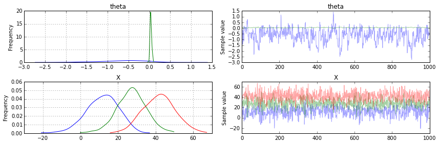
上半分に示した 'theta'（特に青線...theta[0]）の変動の大きさが気になった．

PyMC3 Simulationの収束判断

MCMC(Markov chain Monte Carlo) 計算の収束判断をするやり方はいくつかあるが，まず，Gewekeの方法を試してみた．内容は，MCMC processの前半10%の状況と後半50%の状況を比較することで，プロセスの遷移が収まっているかどうかを調べるというもの（らしい）．PyMC3 でもこの判断機能(pymc3.geweke())はサポートされていた．

# Geweke's Diag.
gwk_out = pm.geweke(trace)
plt.plot(gwk_out['theta'][0][:,0], gwk_out['theta'][0][:,1])
plt.plot(gwk_out['theta'][1][:,0], gwk_out['theta'][1][:,1])
plt.ylim(-2.2, 2.2) ; plt.grid(True)

Fig. Geweke's diag. (theta's Z-value(left), X's Z-value(right))

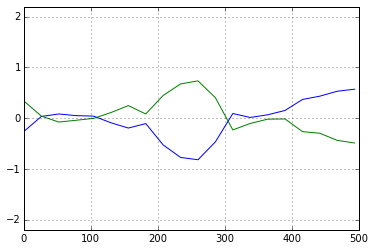
PyMCの（前バージョンの）ドキュメントには，+/-2.0の範囲に入れば収束とみなせると説明があるが，別の情報では +/-1.0 が判断基準，とあった．上図は，いずれにしても「収束」と判断できるものである．

次にAuto-correlation（自己回帰）を調べる方法にtryした．PyMC3にautocorrplot() というものがあったのでそれを使おうとしたのだが，"ValueError: object too deep for desired array” とのことでうまく行かなかった．（まだ，サポートされていない機能らしい．．．）そこで，代わりにmatplotlibのmatplotlib.pyplot.acorr() の機能を用いた．

# for 'theta'
plt.figure(figsize=(10,4))
plt.subplot(121)
plt.acorr(trace['theta'][:,0], detrend=mlab.detrend_mean, maxlags=500)
plt.subplot(122)
plt.acorr(trace['theta'][:,1], detrend=mlab.detrend_mean, maxlags=500)

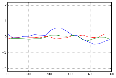
Fig. Autocorrelation plot of 'theta'

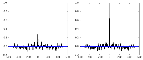
Fig. Autocorrelation plot of 'X'

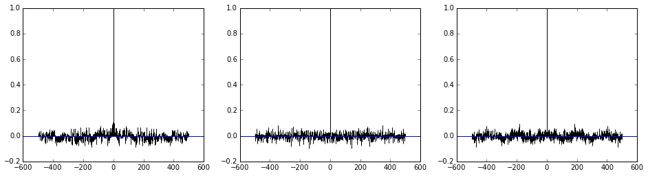
遷移状態を経た後のMCMC processは，互いに（stepの前後）で独立している，という性質をこのplotで確認している．上の図では近接したところを除いて相関が低くなっているので，「収束」とみなせる状況といえる．（収束前では，もっとbroadな線のパターンが観測されるとのこと．針のようなパターンならOK．）

Simulation結果の考察

Logistic Regressionの回帰パラメータをMCMCで推定することを行ったが，今回，パラメータとして'theta'と'X'があった．この結果をうまくVisual化するのにどうするかについて悩んだが，Logistic関数の線形予測子の係数である'theta'の方に着目して作図してみた．

Fig. "Air" example. Logistic regression

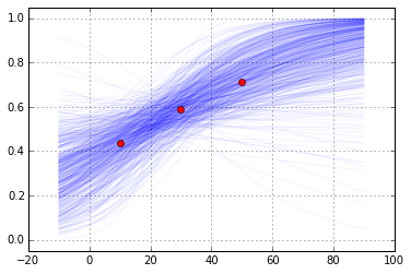
(線の濃さが，「見栄え」に大きく関わります...）

作図のcodeは以下の通り．

def invlogit_np(x):
  return 1.0 / (1.0 + np.exp(-x))

def my_fitting_plot(th0, th1, alpha=0.1):
     x_plot = np.linspace(-10, 90, 50)
     y_plot = invlogit_np(th0 + th1 * x_plot)
     plt.plot(x_plot, y_plot, color='blue', alpha=alpha)

y_i = np.array([21, 20, 15])  # y initial values
y_n_r = y_i * 1.0 / n
for i in range(0, len(trace['theta']), (len(trace['theta'])/250)):  
     my_fitting_plot(trace['theta'][i][0], trace['theta'][i][1], alpha=0.1)
plt.plot(z, y_n_r, 'o', c='r')
plt.ylim(-0.05, 1.05)
plt.grid(True)

青線はfitしたLogistic関数，赤のプロットは問題で与えられた３水準のデータである．

また，今回，BUGS Exampleの例題に提示されていた解答，R(R2jags)による計算，PyMC3による計算を行ったが，その結果を比較したものが下の図である．

Fig. Simulation result comparison ('X')

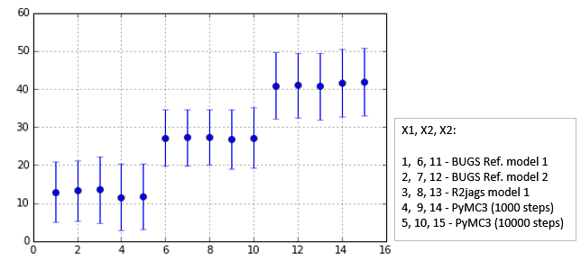
Fig. Simulation result comparison ('theta1')

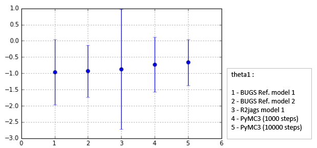
Fig. Simulationresult comparison ('theta2')

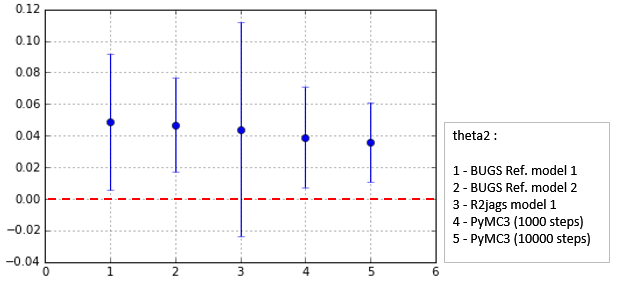
'X'については各計算結果は，概略一致している．しかし，'theta1', 'theta2'については，No.3のR2jagsのsigma値が他の結果より大きくなってしまっている．この計算については見直しが必要のようである．PyMC3については，Refernce結果と整合がとれており大丈夫そうである．

他に注目するポイントとしては，theta2 (theta[1] in python code) の計算結果である．これは，平均値mu が大体 0.05, sigma値(sd)が大体 0.05 である．Traceplot (thetaの緑線の方）をよく見るとわかるが，分布の下の方が，0.0より小さく負の値になっている．theta2は，Logistic関数の右辺のxにかかる係数であることから，これが負の値になると関数の線の向きが（右肩下がりに）変わる特徴がある．実際にLogistic regressionのplot（青色のもやもやplot）でも少数本，このような特徴をもった（右肩下がりの）線が観察できる．（他のほとんどの線は，右肩上がりの典型的なパターンである．）

まとめ

BUGS Exampleにあった"Air"の例題をPyMC3で解いてみた．今回やや複雑なモデルであったが，BUGSのmodelスクリプトを参考にpythonのcodeを作成できた．
前記事でも書いたが，やはりPyMC3のドキュメントは不足していると感じた．（できれば早く整備して欲しい．）
MCMCの収束診断については，現在用意されているtoolでも可能ということが分かった．（Autocorrelation Plotについては，matplotlibのfunctionを使用する．）
R2jagsに関しては，もっと勉強が必要．（PyMC3も同様ですが...）

参考文献(Web site)

OpenBUGS Examples
http://www.openbugs.net/Examples/Air.html
Stan Examples
https://github.com/stan-dev/example-models/wiki
R2jags document (CRAN)
https://cran.r-project.org/web/packages/R2jags/index.html
PyMC3 tutorial
https://pymc-devs.github.io/pymc3/getting_started/
PyMC (previous version) documentation
http://pymc-devs.github.io/pymc/index.html
データ解析のための統計モデリング入門（岩波書店）
https://www.iwanami.co.jp/cgi-bin/isearch?isbn=ISBN978-4-00-006973-1

You get articles that match your needs
You can efficiently read back useful information
You can use dark theme

What you can do with signing up