記事の目的

多次元ガウス分布と、分散共分散行列が未知のときの共役事前分布であるウィシャート分布を使用し、Rを使ってベイズ推定します。
商品Aの購買個数と、商品Bの購買個数の関係を表している分散共分散行列を事後分布で推定します。
参考：ベイズ推論による機械学習入門

0. モデルの説明

1. ライブラリ

library(dplyr)
library(mvtnorm)
library(MCMCpack)
library(ellipse)
set.seed(100)

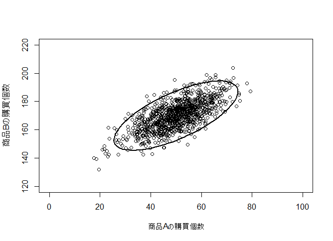
2. 推定する分布

商品Aの購買個数と、商品Bの購買個数は、それぞれ平均が50, 170で、標準偏差が10, 相関係数が0.7の多次元ガウス分布に従います(適当)。
この、真の分布の分散共分散行列を事後分布で推定します。

sigma.true <- matrix(c(10^2, 0.7*10^2, 0.7*10^2, 10^2), ncol=2)
X.true <- rmvnorm(1000, mean = c(50, 170), sigma=sigma.true)
plot(X.true[,1],X.true[,2], xlim = c(0, 100), ylim = c(120, 220), xlab="商品Aの購買個数", ylab="商品Bの購買個数")
ell <-  ellipse(sigma.true) + matrix(rep(c(50,170), each=100), nrow=100) 
lines(ell, lw=2)

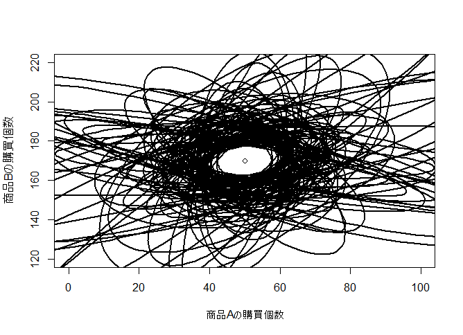
3. 事前分布

事前分布として、多次元ガウス分布の分散共分散行列が未知のときの共役事前分布である逆ウィシャーと分布を指定します。
下図は、逆ウィシャート分布から100個サンプルを取って可視化した図です。

n0 <- 3
w.inv0 <- diag(2)*100
plot(50,170, xlim = c(0, 100), ylim = c(120, 220))
par(new=T)
for(i in 1:100){
  w.pre <- riwish(n0, w.inv0)
  ell <-  ellipse(w.pre) + matrix(rep(c(50,170), each=100), nrow=100) 
  lines(ell, col="black", lw=2)
}

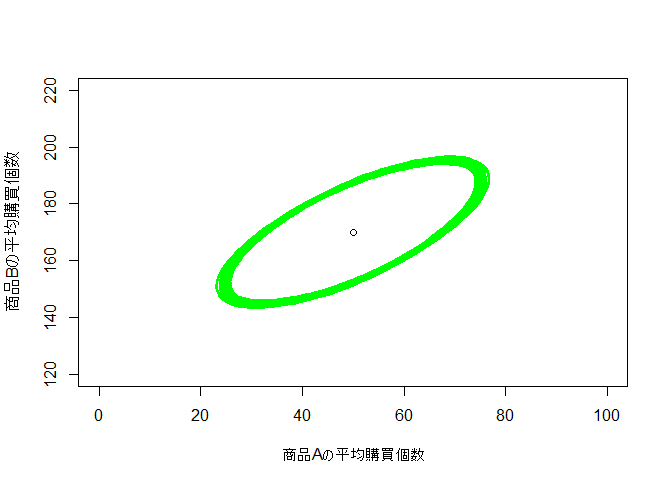
4. 事後分布

真の分布から1000個のサンプルを取って事後分布を推定します。
それぞれの標準偏差が10, 相関係数が0.7である分散共分散行列をうまく推定できていることが分かります。

u <- c(50, 170)
X <- rmvnorm(1000, mean = u, sigma=sigma.true)
n <- nrow(X) + n0
sum.tmp <- 0
for(i in 1:nrow(X)){
  sum.tmp <- sum.tmp + (X[i,]-u) %*% t(X[i,]-u)
}
plot(50,170, xlim = c(0, 100), ylim = c(120, 220), xlab="商品Aの平均購買個数", ylab="商品Bの平均購買個数")
par(new=T)
w.inv <- sum.tmp + w.inv0
for(i in 1:100){
  w.post <- riwish(n, w.inv)
  ell <-  ellipse(w.post) + matrix(rep(c(50,170), each=100), nrow=100) 
  lines(ell, col="green", lw=2)
}

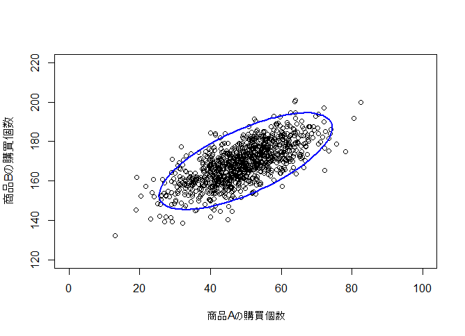
5. 予測分布

予測分布から1000個のサンプルを取って可視化しました。
真の分布をうまく推定できていることが分かります。

u.predict <- u
lambda.predict <- (1-2+n)*solve(w.inv)
n.predict <- 1-2+n
X.predict <- rmvt(1000, delta = u.predict, sigma = solve(lambda.predict), df = n.predict, type="shifted")
plot(X.predict[,1],X.predict[,2], xlim = c(0, 100), ylim = c(120, 220), xlab="商品Aの購買個数", ylab="商品Bの購買個数")
ell <-  ellipse(sigma.true) + matrix(rep(c(50,170), each=100), nrow=100) 
lines(ell, col="blue", lw=2)

多次元ガウス分布 : ウィシャート分布 (ベイズ推定)