記事の目的
正規分布と、分散が未知の時の共役事前分布である正規分布を使用し、Rを使ってベイズ推定を行います。
20男性の身長の分散を事後分布で推定します。
参考:ベイズ推論による機械学習入門
目次
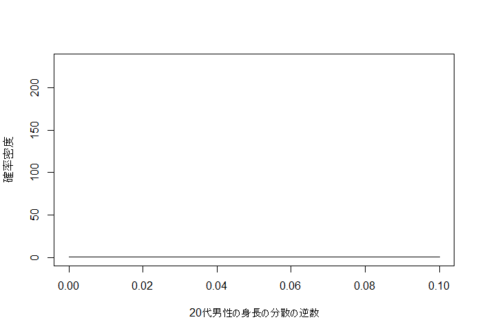
1. モデルの説明
2. 推定する分布
3. 事前分布
4. 事後分布
5. 予測分布
1. モデルの説明
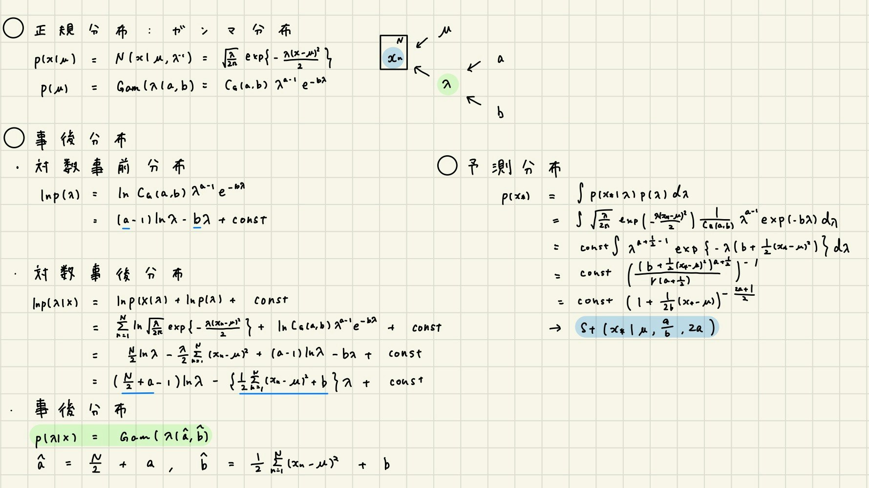
2. 推定する分布
20代男性の身長は、平均が170で標準偏差が10の正規分布に従います(適当)。しかし、僕たちはそれを知りません。
この、真の分布の分散の逆数1/100=0.01を事後分布で推定します。
curve(dnorm(x, 170, 10), 100, 250, xlab="20代男性の身長", ylab="確率密度")
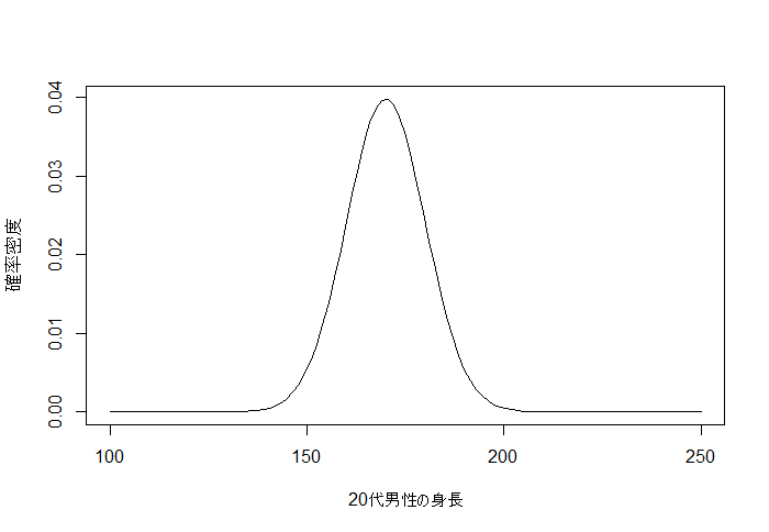
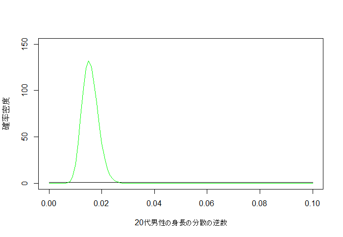
3. 事前分布
事前分布として、正規分布の、分散が未知のときの共役事前分布であるガンマ分布を指定します。
データに適合しやすいように、a0, b0を小さな値で設定します。
a0 <- 1
b0 <- 1
curve(dgamma(x, a0, b0), 0, 0.1, ylim=c(0,150),
      xlab="20代男性の身長の分散の逆数", ylab="確率密度")
4. 事後分布
真の分布から50個のサンプルを取って事後分布を推定します。
事後分布は緑の曲線です。0.01付近が一番出やすいと推定できています。
N <- 50
X <- rnorm(N, 170, 10)
# 事後分布
u0 <- 170
a <- N/2 + a0
b <- ((X-u0) %*% (X-u0))/2 + b0
curve(dgamma(x, a, b), 0, 0.1, add=T, col="green")
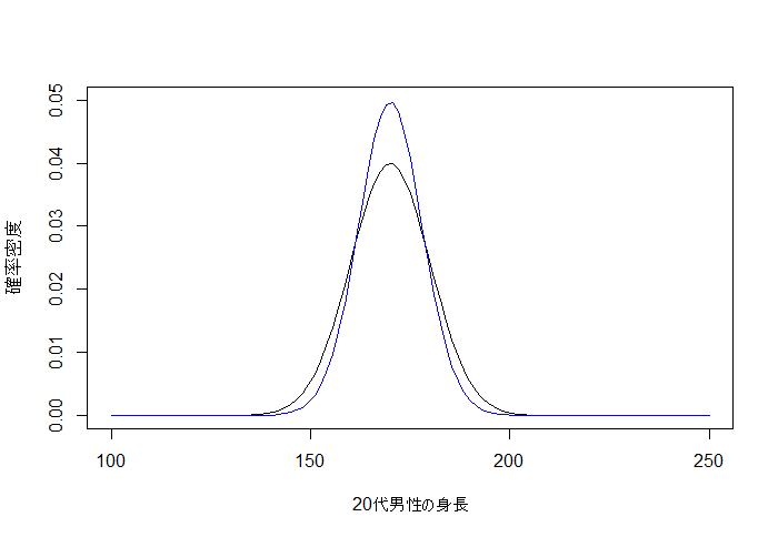
5. 予測分布
少し分散が小さく見積もられていますが、だいたい推定できています。
u.p <- u0
lambda.p <- a/b
n <- 2*a
curve(dnorm(x, 170, 10), 100, 250, ylim=c(0,0.05),xlab="20代男性の身長", ylab="確率密度")
curve(dt(x, df=n)*((1+x^2/n)^((n+1)/2))*sqrt(lambda.p)*((1+lambda.p*(1/n)*(x-u.p)^2)^(-(n+1)/2)), 100, 250,
      add=T, col="blue")