自然言語処理で使う Python スニペット集〜青空文庫データを例に〜 #Python3

事前準備
- パッケージのインポート
- データの取得
ファイル読み書き
前処理ーテキストのノイズ削除
前処理ーJanomeで単語分割
前処理ーMeCabで単語分割
- 単語に分割して特定の品詞のリストを取得
可視化
- 出現回数の多い単語を表示
- 単語の出現回数をプロット
ベクトル化

事前準備

パッケージのインポート

import collections
import glob
import re
import urllib.request
import zipfile

import japanize_matplotlib
import matplotlib.pyplot as plt
import numpy as np
import pandas as pd
import seaborn as sns
from janome.tokenizer import Tokenizer
import MeCab
from sklearn.pipeline import Pipeline
from sklearn.feature_extraction.text import CountVectorizer, TfidfVectorizer
from sklearn.decomposition import TruncatedSVD

データの取得

青空文庫のテキストデータを取得する

url = "https://www.aozora.gr.jp/cards/000148/files/794_ruby_4237.zip"
zip_file = "794_ruby_4237.zip"
urllib.request.urlretrieve(url, zip_file)

zip ファイルがダウンロードされている

$ ls 
794_ruby_4237.zip

ファイル読み書き

zipファイルの解凍・ファイルの読み込み

zip_file = "./794_ruby_4237.zip"
with zipfile.ZipFile(zip_file, "r") as zip:
    zip.extractall() 
    for f in zip.infolist():
        file_name = f.filename
        with open(file_name, "r", encoding="sjis") as file:
            text = file.read()

extractall()：zip ファイルの中身をすべて解凍
infolist()：解凍後のファイルのリスト
open(filename, mode, encoding)：ファイル名、ファイルをどのように使うか、エンコーディングの指定をしてファイルを開く
- mode
  - r：読み出し専用
  - w：書き込み専用
  - a：ファイル追記用
- encoding
  - utf-8
  - sjis
read()：ファイル全体を読み込み、str として返す

ファイルを１行ずつ読み込む

with open(file_name, "r", encoding="sjis") as file:
    for line in file:
        # line：１行

ファイルの保存

with open(file_name, mode='w', encoding="sjis") as file:
    file.write(text)

前処理ーテキストのノイズ削除

正規表現でマッチした箇所を削除

ファイル読み書きで読み込んだテキストに存在するノイズを削除。ノイズ例は下記。

反駁《はんばく》：ルビ
｜：ルビの付く文字列の始まりを特定する記号
［＃「彳＋低のつくり」、第3水準1-84-31］：入力者注。主に外字の説明や、傍点の位置の指定
〔Theatron《テアトロン》, Orche^stra《オルケストラ》, Ske^ne^《スケーネ》, Proske^nion《プロスケニオン》〕：アクセント分解された欧文の囲み

正規表現パターンのコンパイル

regex_list = [
    re.compile(r"《.+?》"), # ルビ
    re.compile(r"｜"), # ルビの付く文字列の始まりを特定する記号
    re.compile(r"［＃.+?］"), # 入力者注
    re.compile(r"〔.+?〕"), # アクセント分解された欧文の囲み
]

re.compile()：正規表現パターンをコンパイル。結果の正規表現オブジェクトを保存して再利用するほうが、一つのプログラムでその表現を何回も使うときに効率的

ちなみに正規表現パターンは https://regex101.com/ を使って確認するといい。

事前に正規表現にマッチする箇所を確認

for regex in regex_list:
    print("regex is ", regex)
    print(re.findall(regex, text))

re.findall(pattern, string)：string 中の pattern による全ての重複しないマッチを、文字列のリストとして返す

正規表現パターンにマッチする箇所を取り除く

cleaned_text = text
for regex in regex_list:
    cleaned_text = regex.sub("", cleaned_text)

数字を0に置換

数字に情報が無い場合は、全て0等に置換する

数字があるテキスト部分

下に２の字が出た。野々宮君がまた「どうです」と聞いた。「２の字が見えます」と言うと、「いまに動きます」と言いながら向こうへ回って何かしているようであった。
　やがて度盛りが明るいなかで動きだした。２が消えた。あとから３が出る。そのあとから４が出る。５が出る。

cleaned_text = re.sub(r'\d+', '0', cleaned_text)

下記のように変換される

数字を0に変換したテキスト

下に0の字が出た。野々宮君がまた「どうです」と聞いた。「0の字が見えます」と言うと、「いまに動きます」と言いながら向こうへ回って何かしているようであった。
　やがて度盛りが明るいなかで動きだした。0が消えた。あとから0が出る。そのあとから0が出る。0が出る。

半角・全角スペース、改行コードを削除

# 改行コード
cleaned_text = re.sub("\n", "", cleaned_text)
# 半角スペース
cleaned_text = re.sub(" ", "", cleaned_text)
# 全角スペース
cleaned_text = re.sub("　", "", cleaned_text)

正規表現にマッチした部分で分割

本文以外の箇所を削除。具体的には下記。

テキスト冒頭の 【テキスト中に現れる記号について】部分
テキスト末尾の 底本部分

テキスト冒頭の【テキスト中に現れる記号について】部分

三四郎
夏目漱石

-------------------------------------------------------
【テキスト中に現れる記号について】

《》：ルビ
（例）頓狂《とんきょう》

｜：ルビの付く文字列の始まりを特定する記号
（例）福岡県｜京都郡《みやこぐん》

［＃］：入力者注　主に外字の説明や、傍点の位置の指定
　　　（数字は、JIS X 0213の面区点番号またはUnicode、底本のページと行数）
（例）※［＃「魚＋師のつくり」、第4水準2-93-37］

〔〕：アクセント分解された欧文をかこむ
（例）〔ve'rite'《ヴェリテ》 vraie《ヴレイ》.〕
アクセント分解についての詳細は下記URLを参照してください
http://www.aozora.gr.jp/accent_separation.html
-------------------------------------------------------

テキスト末尾の底本部分

底本：「三四郎」角川文庫クラシックス、角川書店
　　　1951（昭和26）年10月20日初版発行
　　　1997（平成9）年6月10日127刷
初出：「朝日新聞」
　　　1908（明治41）年9月1日〜12月29日
入力：古村充
校正：かとうかおり
2000年7月1日公開
2014年6月19日修正
青空文庫作成ファイル：
このファイルは、インターネットの図書館、青空文庫（http://www.aozora.gr.jp/）で作られました。入力、校正、制作にあたったのは、ボランティアの皆さんです。

cleaned_text = re.split(r'-{50,}', cleaned_text)[2]
cleaned_text = re.split(r'底本：', cleaned_text)[0]

re.split()：第１引数に正規表現パターン、第２引数に対象の文字列を指定することで、正規表現にマッチした文字列で分割されたリストを受け取る
- re.split(r'-{50,}', cleaned_text)[2]は、２つ目の------------------------------------------------------- 以降のテキストを取得
- re.split(r'底本：', cleaned_text)[0]は、底本：より前のテキストを取得

ファイルに書き出してノイズが削除されていることを確認

with open("./sanshiro_cleaned.txt", mode='w', encoding="sjis") as file:
    file.write(cleaned_text)

参考リンク

前処理ーJanomeで単語分割

単語に分割してそのままの形のリストを取得

t = Tokenizer()
tokenized_text = [token.surface for token in t.tokenize(cleaned_text)]
print(tokenized_text)

surface：文字列の中で使われているそのままの形を取得

出力

[ 'うとうと', 'と', 'し', 'て', '目', 'が', 'さめる', 'と', '女', 'は', 'いつのまにか', '、', '隣', 'の', 'じいさん', 'と'・・・]

単語に分割して原型のリストを取得

t = Tokenizer()
base_tokenized_text = [token.base_form for token in t.tokenize(cleaned_text)]
print(base_tokenized_text)

base_form：単語の原型を取得

出力

['うとうと', 'として', '目', 'が', 'さめる', 'と', '女', 'は', 'いつのまにか', '、', '隣', 'の', 'じいさん', 'と'・・・]

単語に分割して特定の品詞のリストを取得

動詞と名詞のみ取得する場合

t = Tokenizer()
pos_list = ["動詞", "名詞"]
filtered_tokenized_text = [token.surface for token in t.tokenize(cleaned_text) if token.part_of_speech.split(',')[0] in pos_list]
filtered_tokenized_text

part_of_speech：品詞,品詞細分類1,品詞細分類2,品詞細分類3という文字列を取得

Out

['うとうと', '目', 'さめる', '女', '隣', 'じいさん', '話', '始め', 'いる', 'じいさん', '前', '前', '駅', '乗っ', 'いなか者', '発車', 'ぎわに'・・・]

参考リンク

Python, Janomeで日本語の形態素解析、分かち書き（単語分割）

前処理ーMeCabで単語分割

単語に分割して特定の品詞のリストを取得

pos_list = ["名詞", "動詞", "形容詞"]
def wakati(text):
    tagger = MeCab.Tagger('')
    tagger.parse('') 
    node = tagger.parseToNode(text)
    word_list = []
    while node:
        pos = node.feature.split(",")[0]
        if pos in pos_list:
            word = node.surface
            word_list.append(word)
        node = node.next
    return " ".join(word_list)

Tagger()：分割に使用する辞書の形式を指定。新語にも対応しているmecab-ipadic-neologd を指定することが多い

filtered_tokenized_text = []
cleaned_text_list = cleaned_text.split('。')
for cleaned_text in cleaned_text_list:
    filtered_tokenized_text.append(wakati(cleaned_text))
print(filtered_tokenized_text)

Out

['一 うとうと 目 さめる 女 隣 じいさん 話 始め いる',
 'じいさん 前 前 駅 乗っ いなか者',
 '発車 ぎわ 頓狂 声 出し 駆け込ん 来 肌 ぬい 思っ 背中 灸 あと あっ 三四郎 記憶 残っ いる',
 'じいさん 汗 ふい 肌 入れ 女 隣 腰 かけ 注意 し 見 い',
 '女 京都 相乗り',
 '乗っ 時 三 四 郎 目 つい',
 '一色 黒い',
 '三四郎 九州 山陽 線 移っ 京 大阪 近づい 来る うち 女 色 白く なる 故郷 遠のく よう 哀れ 感じ い',
 '女 車 室 いっ 来 時 異性 味方 得 心持ち し',
 '女 色 九州 色',
 '三輪田 光 さん 色',
 '国 立つ ぎわ 光 さん うるさい 女',

 <以下続く>

参考リンク

Python3×日本語：自然言語処理の前処理まとめ

可視化

出現回数の多い単語を表示

動詞、名詞の単語で出現回数トップ10を出力

n = 10
cnt = collections.Counter(' '.join(filtered_tokenized_text).split(' '))
cnt.most_common(n)

出力

[('いる', 997),
 ('し', 913),
 ('三四郎', 903),
 ('の', 510),
 ('ある', 503),
 ('人', 484),
 ('い', 465),
 ('よう', 395),
 ('女', 382),
 ('三', 373)]

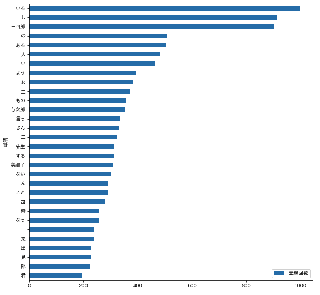
単語の出現回数をプロット

動詞、名詞の単語で出現回数トップ30を描画

n = 30
df_count = pd.DataFrame(cnt.most_common(n), columns=["単語", "出現回数"])
df_count = df_count.set_index("単語")
df_count = df_count.sort_values(by="出現回数", ascending=True)
df_count.plot.barh(y="出現回数", figsize=(10,10))
plt.savefig("出現回数の多い単語.png")

参考リンク

Pythonで自分のどんなツイートが「いいね」されやすいかを分析してみた

ベクトル化

単語に分割して特定の品詞のリストを取得で取得したfiltered_tokenized_textを利用してベクトル化を行う。

print(filtered_tokenized_text)

Out

['一 うとうと 目 さめる 女 隣 じいさん 話 始め いる',
 'じいさん 前 前 駅 乗っ いなか者',
 '発車 ぎわ 頓狂 声 出し 駆け込ん 来 肌 ぬい 思っ 背中 灸 あと あっ 三四郎 記憶 残っ いる',
 'じいさん 汗 ふい 肌 入れ 女 隣 腰 かけ 注意 し 見 い',
 '女 京都 相乗り',
 '乗っ 時 三 四 郎 目 つい',
 '一色 黒い',
 '三四郎 九州 山陽 線 移っ 京 大阪 近づい 来る うち 女 色 白く なる 故郷 遠のく よう 哀れ 感じ い',
 '女 車 室 いっ 来 時 異性 味方 得 心持ち し',
 '女 色 九州 色',
 '三輪田 光 さん 色',
 '国 立つ ぎわ 光 さん うるさい 女',
<以下続く>

Bag of Words

各文に含まれる単語を column、文を row とすると単語の出現回数を要素とした行列形式に変換する方式を Bag of Words という。文に単語が何回含まれているかのみが考慮されるため、単語の現れる順番や文脈は等はもちろん考慮されない。

vectorizer = CountVectorizer(token_pattern='(?u)\\b\\w+\\b', max_features=10)
X = vectorizer.fit_transform(filtered_tokenized_text)
X

scipy.sparse.csr_matrix が返ってくる。これは疎行列を効率的に扱うクラスでメモリ使用量が少なく処理速度も高速になる。

Out

<5904x10 sparse matrix of type '<class 'numpy.int64'>'
    with 5644 stored elements in Compressed Sparse Row format>

X.toarray()

toarray()でnumpy.ndarrayに変換することで確認することは可能。しかし scikit-learn などのライブラリでは、疎行列のままインプットできるので、あえてtoarray()する必要はない。

Out

[[0 0 1 ... 0 0 1]
 [0 0 0 ... 0 0 0]
 [0 0 1 ... 1 0 0]
 ...
 [0 0 0 ... 1 0 2]
 [0 0 0 ... 0 0 0]
 [0 0 0 ... 0 0 0]]

print(f'{X.toarray().shape[0]} rows and {X.toarray().shape[1]} columns')

確かに10 columns になっていることがわかる

Out

5904 rows and 10 columns

token_pattern='(?u)\\b\\w+\\b'
- 1文字以上の文字を含める
- デフォルトのr'(?u)\b\w\w+\b' だと2文字以上の文字が対象になる
max_features=10
- 上位10個のの出現回数の単語を含める

Bag of Words - 単語とインデックスの表示

vectorizer.vocabulary_

Out

{'ある': 0,
 'い': 1,
 'いる': 2,
 'し': 3,
 'の': 4,
 'よう': 5,
 '三': 6,
 '三四郎': 7,
 '人': 8,
 '女': 9}

TFIDF

TFIDF とは、ある文書における単語の出現頻度と逆文書頻度（各文書で）の積で、文章中の単語の重要度を測る手法。

Term Frequency(TF)は、それぞれの単語の文書内での出現頻度
Inverse Document Freaquency(IDF)は、ある単語が全文書の中のどれだけの文書で出現したかの逆数

多くの文書に出現する語の重要度を下げる働きをするため、文書中に含まれる単語の重要度を評価することができる。

tfidf_{i,j} = tf_{i,j} * idf_{i,j}

vectorizer = TfidfVectorizer(token_pattern='(?u)\\b\\w+\\b', max_features=10)
X = vectorizer.fit_transform(filtered_tokenized_text)
X

CountVectorizer と同様に scipy.sparse.csr_matrix が返ってるが、sparse matrix の type が numpy.float64となっている。

Out

<5904x10 sparse matrix of type '<class 'numpy.float64'>'
    with 5644 stored elements in Compressed Sparse Row format>

同様にtoarray()でnumpy.ndarrayに変換することで確認することは可能。

X.toarray()

Out

[[0.         0.         0.59910191 ... 0.         0.         0.80067278]
 [0.         0.         0.         ... 0.         0.         0.        ]
 [0.         0.         0.70052464 ... 0.71362821 0.         0.        ]
 ...
 [0.         0.         0.         ... 0.35613389 0.         0.93443494]
 [0.         0.         0.         ... 0.         0.         0.        ]
 [0.         0.         0.         ... 0.         0.         0.        ]]

Okapi BM25

TFIDF と同様に単語の重要度を測る手法だが、TF, IDF値に加えて、DF(Document Frequency) を使用して、文ごとの単語数の違いを吸収する。Scikit Learn に実装されていないため、BM25Transformer、テーブルデータ向けの自然言語特徴抽出術を参考にする。

from __future__ import absolute_import, division, print_function, unicode_literals
import numpy as np
import scipy.sparse as sp
from sklearn.base import BaseEstimator, TransformerMixin
from sklearn.utils.validation import check_is_fitted
from sklearn.feature_extraction.text import _document_frequency

class BM25Transformer(BaseEstimator, TransformerMixin):
    """
    Parameters
    ----------
    use_idf : boolean, optional (default=True)
    k1 : float, optional (default=2.0)
    b : float, optional (default=0.75)
    References
    ----------
    Okapi BM25: a non-binary model - Introduction to Information Retrieval
    http://nlp.stanford.edu/IR-book/html/htmledition/okapi-bm25-a-non-binary-model-1.html
    """
    def __init__(self, use_idf=True, k1=2.0, b=0.75):
        self.use_idf = use_idf
        self.k1 = k1
        self.b = b

    def fit(self, X):
        """
        Parameters
        ----------
        X : sparse matrix, [n_samples, n_features]
            document-term matrix
        """
        if not sp.issparse(X):
            X = sp.csc_matrix(X)
        if self.use_idf:
            n_samples, n_features = X.shape
            df = _document_frequency(X)
            idf = np.log((n_samples - df + 0.5) / (df + 0.5))
            self._idf_diag = sp.spdiags(idf, diags=0, m=n_features, n=n_features)
        return self

    def transform(self, X, copy=True):
        """
        Parameters
        ----------
        X : sparse matrix, [n_samples, n_features]
            document-term matrix
        copy : boolean, optional (default=True)
        """
        if hasattr(X, 'dtype') and np.issubdtype(X.dtype, np.float):
            X = sp.csr_matrix(X, copy=copy)
        else:
            X = sp.csr_matrix(X, dtype=np.float64, copy=copy)

        n_samples, n_features = X.shape
        dl = X.sum(axis=1)
        sz = X.indptr[1:] - X.indptr[0:-1]
        rep = np.repeat(np.asarray(dl), sz)
        # Average document length
        # Scalar value
        avgdl = np.average(dl)
        # Compute BM25 score only for non-zero elements
        data = X.data * (self.k1 + 1) / (X.data + self.k1 * (1 - self.b + self.b * rep / avgdl))
        X = sp.csr_matrix((data, X.indices, X.indptr), shape=X.shape)

        if self.use_idf:
            check_is_fitted(self, '_idf_diag', 'idf vector is not fitted')

            expected_n_features = self._idf_diag.shape[0]
            if n_features != expected_n_features:
                raise ValueError("Input has n_features=%d while the model"
                                 " has been trained with n_features=%d" % (
                                     n_features, expected_n_features))
            X = X * self._idf_diag

        return X

bm25_vectorizer = Pipeline(steps=[
    ("CountVectorizer", CountVectorizer()),
    ("BM25Transformer", BM25Transformer())
])
X = bm25_vectorizer.fit_transform(filtered_tokenized_text)
X

Out

<5904x5624 sparse matrix of type '<class 'numpy.float64'>'
    with 31145 stored elements in Compressed Sparse Row format>

X.toarray()

Out

array([[0., 0., 0., ..., 0., 0., 0.],
       [0., 0., 0., ..., 0., 0., 0.],
       [0., 0., 0., ..., 0., 0., 0.],
       ...,
       [0., 0., 0., ..., 0., 0., 0.],
       [0., 0., 0., ..., 0., 0., 0.],
       [0., 0., 0., ..., 0., 0., 0.]])

LSI

vectorizer = TfidfVectorizer(token_pattern='(?u)\\b\\w+\\b', max_features=10)
X = vectorizer.fit_transform(filtered_tokenized_text)
num_components = 10
lsa = TruncatedSVD(n_components=num_components, n_iter=100, random_state=42)
X = lsa.fit_transform(X)
X

Out

array([[ 0.13374591, -0.01506388,  0.04424599, ...,  0.050291  ,
        -0.04069491, -0.10466084],
       [ 0.03117341,  0.01394953, -0.01074761, ...,  0.01447406,
         0.0014964 , -0.01871558],
       [ 0.11293278, -0.04016784, -0.04309673, ...,  0.04191944,
        -0.04320969,  0.0040198 ],
       ...,
       [ 0.13174625, -0.04839639, -0.07971575, ...,  0.07970447,
        -0.09604262, -0.21915453],
       [ 0.02379   , -0.00061748, -0.0028468 , ...,  0.01337834,
        -0.00111179, -0.01335078],
       [ 0.        ,  0.        ,  0.        , ...,  0.        ,
         0.        ,  0.        ]])

Latent Semantic Indexing using Scikit-Learn

自然言語処理で使う Python スニペット集〜青空文庫データを例に〜

目次

事前準備

パッケージのインポート

データの取得

ファイル読み書き

zipファイルの解凍・ファイルの読み込み

ファイルを１行ずつ読み込む

ファイルの保存

前処理ーテキストのノイズ削除

正規表現でマッチした箇所を削除

正規表現パターンのコンパイル

事前に正規表現にマッチする箇所を確認

正規表現パターンにマッチする箇所を取り除く

数字を0に置換

半角・全角スペース、改行コードを削除

正規表現にマッチした部分で分割

参考リンク

前処理ーJanomeで単語分割

単語に分割してそのままの形のリストを取得

単語に分割して原型のリストを取得

単語に分割して特定の品詞のリストを取得

参考リンク

前処理ーMeCabで単語分割

単語に分割して特定の品詞のリストを取得

参考リンク

可視化

出現回数の多い単語を表示

単語の出現回数をプロット

参考リンク

ベクトル化

Bag of Words

Bag of Words - 単語とインデックスの表示

TFIDF

Okapi BM25

LSI

fasttext

Word2Vec

Doc2Vec

自然言語処理で使う Python スニペット集 〜 青空文庫データを例に 〜

目次

事前準備

パッケージのインポート

データの取得

ファイル読み書き

zipファイルの解凍・ファイルの読み込み

ファイルを１行ずつ読み込む

ファイルの保存

前処理ーテキストのノイズ削除

正規表現でマッチした箇所を削除

正規表現パターンのコンパイル

事前に正規表現にマッチする箇所を確認

正規表現パターンにマッチする箇所を取り除く

数字を0に置換

半角・全角スペース、改行コードを削除

正規表現にマッチした部分で分割

参考リンク

前処理ーJanomeで単語分割

単語に分割してそのままの形のリストを取得

単語に分割して原型のリストを取得

単語に分割して特定の品詞のリストを取得

参考リンク

前処理ーMeCabで単語分割

単語に分割して特定の品詞のリストを取得

参考リンク

可視化

出現回数の多い単語を表示

単語の出現回数をプロット

参考リンク

ベクトル化

Bag of Words

Bag of Words - 単語とインデックスの表示

TFIDF

Okapi BM25

LSI

fasttext

Word2Vec

Doc2Vec

自然言語処理で使う Python スニペット集〜青空文庫データを例に〜