Google Colabで実践する中心性指標の計算（Eigenvector / PageRank / Katz）

はじめに

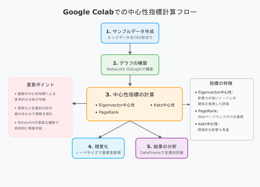
Google Colab上で、**中心性指標（Eigenvector / PageRank / Katz）**を計算する方法を紹介します。サンプルデータをコード内で作成し、全体の流れを1つのノートブックで完結させます。

使用ライブラリ

• NetworkX: グラフ解析用ライブラリ
• Matplotlib: グラフ描画用
• pandas: CSVファイルの操作用

Google Colab環境で必要に応じて以下のコードでインストールできます：

!pip install networkx==3.0 matplotlib pandas

1. サンプルデータの作成

まず、プログラム内でサンプルのエッジデータ（ノードの接続情報）を作成し、CSVファイルとして保存します。

import pandas as pd

# サンプルデータをリスト形式で作成
edges_data = [
    {'source': 'A', 'target': 'B'},
    {'source': 'B', 'target': 'C'},
    {'source': 'B', 'target': 'D'},
    {'source': 'C', 'target': 'D'},
    {'source': 'C', 'target': 'E'},
    {'source': 'D', 'target': 'A'},
    {'source': 'E', 'target': 'B'},
    {'source': 'E', 'target': 'C'},
]

# DataFrame化してCSVに保存
df_edges = pd.DataFrame(edges_data)
df_edges.to_csv("sample_edges.csv", index=False)

# 作成したCSVを確認
!head sample_edges.csv

2. グラフの構築と可視化

作成したCSVデータを読み込み、有向グラフを構築します。NetworkXを利用してノードやエッジを可視化します。

import networkx as nx
import matplotlib.pyplot as plt
import csv

# 有向グラフを作成
G = nx.DiGraph()

# CSVファイルからエッジを追加
with open("sample_edges.csv", "r") as f:
    reader = csv.DictReader(f)
    for row in reader:
        G.add_edge(row['source'], row['target'])

# グラフのノード・エッジ情報を確認
print("Nodes:", G.nodes())
print("Edges:", G.edges())

# グラフの可視化
pos = nx.spring_layout(G, seed=42)
nx.draw(G, pos, with_labels=True, node_color='lightblue', arrows=True)
plt.title("Sample Directed Graph")
plt.show()

3. 各種中心性指標の計算

3.1 Eigenvector 中心性

eigen_centrality = nx.eigenvector_centrality_numpy(G)
print("=== Eigenvector Centrality ===")
for node, score in eigen_centrality.items():
    print(f"  Node {node}: {score:.4f}")

3.2 PageRank

pagerank = nx.pagerank(G, alpha=0.85)
print("\n=== PageRank ===")
for node, score in pagerank.items():
    print(f"  Node {node}: {score:.4f}")

3.3 Katz 中心性（修正後）

NetworkX 3.0以降に対応する方法でKatz中心性を計算します。隣接行列を使用し、固有値と固有ベクトルを計算します。

import numpy as np

# 有向グラフの隣接行列を取得
A = nx.adjacency_matrix(G).astype(float)  # 隣接行列をスパース行列として取得
A_dense = A.toarray()  # 密行列に変換

# Katz中心性の計算
eigenvalues, eigenvectors = np.linalg.eig(A_dense)  # 固有値・固有ベクトルを計算
katz_centrality = {node: eigenvectors[i, 0] for i, node in enumerate(G.nodes())}  # 固有ベクトルの最初の要素を取得

print("\n=== Katz Centrality (modified) ===")
for node, score in katz_centrality.items():
    print(f"  Node {node}: {score:.4f}")

4. 結果をDataFrameにまとめる

各中心性指標をDataFrameにまとめて表示します。

df_centrality = pd.DataFrame({
    'Node': list(G.nodes()),
    'Eigenvector': [eigen_centrality[n] for n in G.nodes()],
    'PageRank': [pagerank[n] for n in G.nodes()],
    'Katz': [katz_centrality[n] for n in G.nodes()]
})

df_centrality_sorted = df_centrality.sort_values('PageRank', ascending=False)
print("\n=== DataFrame(sorted by PageRank) ===")
print(df_centrality_sorted)

5. 中心性指標を可視化に反映させる

PageRankに基づいてノードのサイズを変化させ、グラフを可視化します。

node_size = [pagerank[node] * 2000 for node in G.nodes()]

plt.figure(figsize=(6, 6))
nx.draw(
    G,
    pos,
    with_labels=True,
    node_color='lightblue',
    node_size=node_size,
    arrows=True,
    arrowstyle='->',
    arrowsize=15
)
plt.title("Node Size by PageRank")
plt.show()

まとめ

• Eigenvector 中心性: 重要なノードと繋がるノードがさらに重要視されます。
• PageRank: Google の検索エンジンに応用されるアルゴリズム。ランダムサーファーモデルをベースにしています。
• Katz 中心性: 減衰率やバイアスを用いて、直接・間接的なつながりを評価します。

Google Colab を活用することで、簡単にネットワークデータの解析が可能です。ぜひ実際のデータに適用してみてください！

実装例

import pandas as pd
import networkx as nx
import matplotlib.pyplot as plt
import numpy as np
import csv

# 1. サンプルデータの作成
def create_sample_data():
    edges_data = [
        {'source': 'A', 'target': 'B'},
        {'source': 'B', 'target': 'C'},
        {'source': 'B', 'target': 'D'},
        {'source': 'C', 'target': 'D'},
        {'source': 'C', 'target': 'E'},
        {'source': 'D', 'target': 'A'},
        {'source': 'E', 'target': 'B'},
        {'source': 'E', 'target': 'C'},
    ]
    
    # DataFrame化してCSVに保存
    df_edges = pd.DataFrame(edges_data)
    df_edges.to_csv("sample_edges.csv", index=False)
    return df_edges

# 2. グラフの構築と基本可視化
def create_and_visualize_graph(csv_path):
    G = nx.DiGraph()
    
    # CSVファイルからエッジを追加
    with open(csv_path, "r") as f:
        reader = csv.DictReader(f)
        for row in reader:
            G.add_edge(row['source'], row['target'])
    
    # グラフの基本情報を出力
    print("\nグラフ基本情報:")
    print(f"ノード数: {G.number_of_nodes()}")
    print(f"エッジ数: {G.number_of_edges()}")
    print("ノード:", G.nodes())
    print("エッジ:", G.edges())
    
    # グラフの可視化（基本）
    plt.figure(figsize=(8, 6))
    pos = nx.spring_layout(G, seed=42)
    nx.draw(G, pos, with_labels=True, node_color='lightblue', 
            arrows=True, node_size=500, font_size=12)
    plt.title("Sample Directed Graph")
    plt.savefig('basic_graph.png')
    plt.close()
    
    return G, pos

# 3. 各種中心性指標の計算
def calculate_centralities(G):
    # Eigenvector中心性
    eigen_centrality = nx.eigenvector_centrality_numpy(G)
    print("\nEigenvector Centrality:")
    for node, score in eigen_centrality.items():
        print(f"  Node {node}: {score:.4f}")
    
    # PageRank
    pagerank = nx.pagerank(G, alpha=0.85)
    print("\nPageRank:")
    for node, score in pagerank.items():
        print(f"  Node {node}: {score:.4f}")
    
    # Katz中心性
    # 隣接行列を使用した計算
    A = nx.adjacency_matrix(G).astype(float)
    A_dense = A.toarray()
    eigenvalues, eigenvectors = np.linalg.eig(A_dense)
    katz_centrality = {node: abs(eigenvectors[i, 0].real) 
                      for i, node in enumerate(G.nodes())}
    
    print("\nKatz Centrality:")
    for node, score in katz_centrality.items():
        print(f"  Node {node}: {score:.4f}")
    
    return eigen_centrality, pagerank, katz_centrality

# 4. 結果をDataFrameにまとめる
def create_centrality_dataframe(G, eigen_centrality, pagerank, katz_centrality):
    df_centrality = pd.DataFrame({
        'Node': list(G.nodes()),
        'Eigenvector': [eigen_centrality[n] for n in G.nodes()],
        'PageRank': [pagerank[n] for n in G.nodes()],
        'Katz': [katz_centrality[n] for n in G.nodes()]
    })
    
    # PageRankでソート
    df_centrality_sorted = df_centrality.sort_values('PageRank', ascending=False)
    print("\nCentrality Measures (sorted by PageRank):")
    print(df_centrality_sorted)
    
    # CSV形式で保存
    df_centrality_sorted.to_csv('centrality_results.csv', index=False)
    return df_centrality_sorted

# 5. 中心性指標を可視化に反映
def visualize_with_centrality(G, pos, pagerank):
    plt.figure(figsize=(10, 8))
    
    # ノードサイズをPageRankに基づいて設定
    node_size = [pagerank[node] * 3000 for node in G.nodes()]
    
    nx.draw(
        G,
        pos,
        with_labels=True,
        node_color='lightblue',
        node_size=node_size,
        arrows=True,
        arrowsize=20,
        arrowstyle='->',
        font_size=12,
        font_weight='bold'
    )
    
    plt.title("Node Size Reflects PageRank Centrality")
    plt.savefig('centrality_visualization.png')
    plt.close()

def main():
    # 1. データ作成
    print("1. サンプルデータの作成...")
    df_edges = create_sample_data()
    print("エッジデータ:")
    print(df_edges)
    
    # 2. グラフ構築
    print("\n2. グラフの構築と可視化...")
    G, pos = create_and_visualize_graph("sample_edges.csv")
    
    # 3. 中心性指標の計算
    print("\n3. 中心性指標の計算...")
    eigen_centrality, pagerank, katz_centrality = calculate_centralities(G)
    
    # 4. 結果のまとめ
    print("\n4. 結果のDataFrame化...")
    df_centrality = create_centrality_dataframe(
        G, eigen_centrality, pagerank, katz_centrality
    )
    
    # 5. 中心性を反映した可視化
    print("\n5. 中心性を反映した可視化...")
    visualize_with_centrality(G, pos, pagerank)
    
    print("\n処理完了!")
    print("出力ファイル:")
    print("- sample_edges.csv: エッジデータ")
    print("- basic_graph.png: 基本グラフ可視化")
    print("- centrality_results.csv: 中心性指標の計算結果")
    print("- centrality_visualization.png: PageRankを反映したグラフ可視化")

if __name__ == "__main__":
    main()

出力例:

1. サンプルデータの作成...
エッジデータ:
  source target
0      A      B
1      B      C
2      B      D
3      C      D
4      C      E
5      D      A
6      E      B
7      E      C

2. グラフの構築と可視化...

グラフ基本情報:
ノード数: 5
エッジ数: 8
ノード: ['A', 'B', 'C', 'D', 'E']
エッジ: [('A', 'B'), ('B', 'C'), ('B', 'D'), ('C', 'D'), ('C', 'E'), ('D', 'A'), ('E', 'B'), ('E', 'C')]

3. 中心性指標の計算...

Eigenvector Centrality:
  Node A: 0.3766
  Node B: 0.4380
  Node C: 0.4773
  Node D: 0.5871
  Node E: 0.3062

PageRank:
  Node A: 0.2182
  Node B: 0.2622
  Node C: 0.1882
  Node D: 0.2214
  Node E: 0.1100

Katz Centrality:
  Node A: 0.2929
  Node B: 0.4567
  Node C: 0.5240
  Node D: 0.1879
  Node E: 0.6291

4. 結果のDataFrame化...

Centrality Measures (sorted by PageRank):
  Node  Eigenvector  PageRank      Katz
1    B     0.437981  0.262216  0.456667
3    D     0.587132  0.221419  0.187897
0    A     0.376613  0.218207  0.292927
2    C     0.477346  0.188182  0.524038
4    E     0.306191  0.109978  0.629069

5. 中心性を反映した可視化...

処理完了!
出力ファイル:
- sample_edges.csv: エッジデータ
- basic_graph.png: 基本グラフ可視化
- centrality_results.csv: 中心性指標の計算結果
- centrality_visualization.png: PageRankを反映したグラフ可視化