さまざまなグラフ生成方法：データ構造と NetworkX の連携

はじめに

Python の NetworkX ライブラリを使い、Google Colab で試せるハンズオン形式のチュートリアルです。

---

必要なライブラリのインストール

以下を Google Colab 上で実行してください。

!pip install networkx

次に、必要なライブラリをインポートします。

import networkx as nx
import matplotlib.pyplot as plt
%matplotlib inline

---

Python のリスト・タプルからグラフを作る

エッジリストの例

# エッジリストの例(タプルのリスト)
edge_list = [
    ('A', 'B'),
    ('B', 'C'),
    ('C', 'D'),
    ('A', 'D')
]

# 無向グラフを作成
G1 = nx.Graph()
G1.add_edges_from(edge_list)

# グラフの可視化
nx.draw(G1, with_labels=True)
plt.show()

---

Pandas・CSV を用いたグラフ生成

CSV ファイルの例

以下は CSV ファイルを作成してエッジ情報を定義する例です。

import pandas as pd

# Google Colab 上での一時 CSV 作成例
csv_text = """source,target
A,B
B,C
C,D
D,A
A,E
"""

with open("edges.csv", "w") as f:
    f.write(csv_text)

df_edges = pd.read_csv("edges.csv")
df_edges

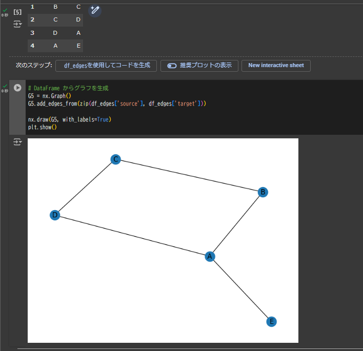
CSV からグラフ生成

# DataFrame からグラフを生成
G5 = nx.Graph()
G5.add_edges_from(zip(df_edges['source'], df_edges['target']))

nx.draw(G5, with_labels=True)
plt.show()

---

まとめ

• NetworkX を使って、Python の基本データ構造や CSV ファイルからグラフを生成する方法を解説しました。
• Google Colab を使うことで簡単に可視化が可能です。
• ぜひ自身のデータを用いて試してみてください！

実装例: ノートブック

{
    "cells": [
        {
            "cell_type": "markdown",
            "metadata": {},
            "source": [
                "# \u3055\u307e\u3056\u307e\u306a\u30b0\u30e9\u30d5\u751f\u6210\u65b9\u6cd5\uff1a\u30c7\u30fc\u30bf\u69cb\u9020\u3068 NetworkX \u306e\u9023\u643a\n",
                "\n",
                "Python \u306e NetworkX \u30e9\u30a4\u30d6\u30e9\u30ea\u3092\u4f7f\u3044\u3001Google Colab \u3067\u8a66\u305b\u308b\u30cf\u30f3\u30ba\u30aa\u30f3\u5f62\u5f0f\u306e\u30c1\u30e5\u30fc\u30c8\u30ea\u30a2\u30eb\u3067\u3059\u3002"
            ]
        },
        {
            "cell_type": "code",
            "execution_count": null,
            "metadata": {},
            "outputs": [],
            "source": [
                "# \u5fc5\u8981\u306a\u30e9\u30a4\u30d6\u30e9\u30ea\u306e\u30a4\u30f3\u30b9\u30c8\u30fc\u30eb\n",
                "!pip install networkx"
            ]
        },
        {
            "cell_type": "code",
            "execution_count": null,
            "metadata": {},
            "outputs": [],
            "source": [
                "# \u5fc5\u8981\u306a\u30e9\u30a4\u30d6\u30e9\u30ea\u306e\u30a4\u30f3\u30dd\u30fc\u30c8\n",
                "import networkx as nx\n",
                "import matplotlib.pyplot as plt\n",
                "%matplotlib inline"
            ]
        },
        {
            "cell_type": "markdown",
            "metadata": {},
            "source": [
                "## Python \u306e\u30ea\u30b9\u30c8\u30fb\u30bf\u30d7\u30eb\u304b\u3089\u30b0\u30e9\u30d5\u3092\u4f5c\u308b"
            ]
        },
        {
            "cell_type": "code",
            "execution_count": null,
            "metadata": {},
            "outputs": [],
            "source": [
                "# \u30a8\u30c3\u30b8\u30ea\u30b9\u30c8\u306e\u4f8b(\u30bf\u30d7\u30eb\u306e\u30ea\u30b9\u30c8)\n",
                "edge_list = [\n",
                "    ('A', 'B'),\n",
                "    ('B', 'C'),\n",
                "    ('C', 'D'),\n",
                "    ('A', 'D')\n",
                "]\n",
                "\n",
                "# \u7121\u5411\u30b0\u30e9\u30d5\u3092\u4f5c\u6210\n",
                "G1 = nx.Graph()\n",
                "G1.add_edges_from(edge_list)\n",
                "\n",
                "# \u30b0\u30e9\u30d5\u306e\u53ef\u8996\u5316\n",
                "nx.draw(G1, with_labels=True)\n",
                "plt.show()"
            ]
        },
        {
            "cell_type": "markdown",
            "metadata": {},
            "source": [
                "## Pandas\u30fbCSV \u3092\u7528\u3044\u305f\u30b0\u30e9\u30d5\u751f\u6210"
            ]
        },
        {
            "cell_type": "code",
            "execution_count": null,
            "metadata": {},
            "outputs": [],
            "source": [
                "import pandas as pd\n",
                "\n",
                "# Google Colab \u4e0a\u3067\u306e\u4e00\u6642 CSV \u4f5c\u6210\u4f8b\n",
                "csv_text = \"\"\"source,target\n",
                "A,B\n",
                "B,C\n",
                "C,D\n",
                "D,A\n",
                "A,E\n",
                "\"\"\"\n",
                "\n",
                "with open(\"edges.csv\", \"w\") as f:\n",
                "    f.write(csv_text)\n",
                "\n",
                "df_edges = pd.read_csv(\"edges.csv\")\n",
                "df_edges"
            ]
        },
        {
            "cell_type": "code",
            "execution_count": null,
            "metadata": {},
            "outputs": [],
            "source": [
                "# DataFrame \u304b\u3089\u30b0\u30e9\u30d5\u3092\u751f\u6210\n",
                "G5 = nx.Graph()\n",
                "G5.add_edges_from(zip(df_edges['source'], df_edges['target']))\n",
                "\n",
                "nx.draw(G5, with_labels=True)\n",
                "plt.show()"
            ]
        }
    ],
    "metadata": {
        "kernelspec": {
            "display_name": "Python 3",
            "language": "python",
            "name": "python3"
        },
        "language_info": {
            "codemirror_mode": {
                "name": "ipython",
                "version": 3
            },
            "file_extension": ".py",
            "mimetype": "text/x-python",
            "name": "python",
            "nbconvert_exporter": "python",
            "pygments_lexer": "ipython3",
            "version": "3.8.16"
        }
    },
    "nbformat": 4,
    "nbformat_minor": 4
}