統計学の勉強をしていて不偏性と一致性が理解できなかったので、Pythonでシミュレーションして理解してみました。
Pythonも統計学も初心者で勉強のために記事を書いており不適切なことを書いているかもしれないので鵜呑みにしないでください。
不偏性と一致性の違い
大雑把に言って不偏性は平均的に母集団のパラメータと偏りなく一致することを言います。
一致性は、一つの標本に含まれる要素の数を増やしていくと母集団のパラメータと一致することをいいます。
不偏性
θの推定量
\hat{\theta_n} = h(X_1, X_2, ..., X_n)\\
h()は平均や分散などの統計量の関数を表す。
統計量の平均を取ると母集団のパラメータθに近づいていく。
E(\hat{\theta_1}, \hat{\theta_2}, \hat{\theta_3}, ... , \hat{\theta_n})= \theta
一致性
任意の正の定数aに対して、n→∞としたとき推定量θ^が
\hat{\theta_n} = h(X_1, X_2, ...,X_\infty)\\
P(| \hat{\theta_n} - \theta | < a) \longrightarrow 1
n→∞の時、θ^が小さな区間(θ-a, θ+a)の中に落ちる確率が1に近づいていくこと。
シミュレーション
Pythonでシミュレーションをして不偏性と一致性を視覚的に理解したいと思います!
不偏性
import numpy as np
import matplotlib
import matplotlib.pyplot as plt


np.random.seed(20)

eu = [] #不偏分散の期待値のリスト
es = [] #標本分散の期待値のリスト

uv = [] #不偏分散のリスト
sv = [] #標本分散のリスト

for n in range(1, 10000):
   samples = np.random.normal(10, 5, 10) #平均10、標準偏差5の正規乱数を10個生成生成

   uv.append(np.var(samples, ddof = 1))
   sv.append(np.var(samples, ddof = 0))

   eu.append(np.mean(uv))
   es.append(np.mean(sv))


plt.figure(figsize = (15, 10))
plt.axhline(25, ls = "--", color = "red", label ="True")

plt.plot(eu, color = "blue", linewidth = 0.5, label = "Unbiased variance") #Unbiased variance = 不偏分散
plt.plot(es, color = "green", linewidth = 0.5, label = "Sample variance") #Unbiased variance = 標本分散

plt.xlabel("Samples")
plt.ylabel("Variance")
plt.legend(loc = "higher right")
plt.show()
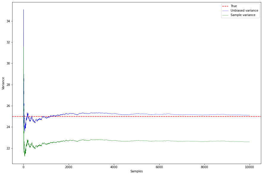
不偏推定量である不偏分散(Unbiased variance)の方が母分散の25に近いですね!
一致性
mean = []

for i in range(1,10000): #標本の要素の数を1から10000
    #平均10、標準偏差5の標本を生成。標本の要素の数は1から10000個に増えていく
    samples = np.random.normal(10, 5, i)

    mean.append(np.mean(samples))

plt.figure(figsize = (15, 10))
plt.axhline(10, ls = "--", color = "red", label ="True")
plt.plot(mean, color = "blue", linewidth = 0.5, label = "Sample mean")

plt.xlabel("Samples")
plt.ylabel("Mean")
plt.legend(loc = "higher right")
plt.show()

一致推定量である標本平均が母平均に近づいていくことがわかりますね!
ちなみに、不偏分散のシミュレーションを見ると、不偏分散と標本分散も一致性を満たすので一定の値に収斂していくことがわかります。