以下は，R 入門のために書かれた

を，Julia ではこんな風になるよということで書いたものである。

R の入門というページは多く存在する。

R に入門しようとしている人 ... Julia にしませんか？

線形モデルによる回帰分析

`llsq()` 関数を用いて単回帰分析

説明変数 x を用いて目的変数 yを予測する。

以下の例で，x, y は実数とするので，簡単のため最初の要素だけ小数点を付けて定義する。

なお，Julia では行末に ; は不要であるが，REPL の場合に評価結果を表示させないために付けることがある。

x = [10., 20, 10, 40, 50, 10, 10, 20, 70];
y = [1., 3, 4, 10, 5, 1, 3, 14, 21];

Julia でも何通りかあるが，MultivariateStats にある llsq() を用いる。¹

using MultivariateStats

また，基本的に llsq() は重回帰分析も行えるので，説明変数はたとえ 1 個（つまり単回帰分析）の場合であっても，n × 1 行列にしておかねばならない。

ベクトル x を reshape() によって行列に変換する。

X = reshape(x, length(y), :);

llsq() はデフォルトで定数項を含めるモデル（y = ax + b）を採用する。²

slope, intercept = llsq(X, y);

戻り値は，傾き(slope) と切片(intercept) である。

上の例に示すように，左辺に slope, intercept と書いておけば，結果がそれぞれの変数に代入される。

println("slope = $slope, intercept = $intercept")

slope = 0.23596491228070177, intercept = 0.5964912280701752

llsq() は傾きと切片の結果しか返さないので，偏回帰係数の有意性検定などをしたければ，自分でプログラムしなければならない。

`GLM` による分析

GLM によれば，R と同じような感じで回帰分析を行える。

using GLM

ただし，データはデータフレームにしておく必要がある。

using DataFrames
df = DataFrame(x=x, y=y)

9 rows × 2 columns

	x	y
	Float64	Float64
1	10.0	1.0
2	20.0	3.0
3	10.0	4.0
4	40.0	10.0
5	50.0	5.0
6	10.0	1.0
7	10.0	3.0
8	20.0	14.0
9	70.0	21.0

R の lm() 関数と同じような書き方で分析できる。

results = lm(@formula(y ~ x), df);
println(results)

StatsModels.DataFrameRegressionModel{LinearModel{LmResp{Vector{Float64}}, DensePredChol{Float64, LinearAlgebra.Cholesky{Float64, Matrix{Float64}}}}, Matrix{Float64}}

Formula: y ~ 1 + x

Coefficients:
────────────────────────────────────────────────────
             Estimate  Std.Error   t value  Pr(>|t|)
────────────────────────────────────────────────────
(Intercept)  0.596491  2.60529    0.228954    0.8254
x            0.235965  0.0773885  3.04909     0.0186
────────────────────────────────────────────────────

結果も同じように表示される。

多分，R の関数を呼んでいるのだろう。
偏回帰係数（定数項），それらの標準誤差，有意性検定の t 値および P 値が表示される。

個別の統計量は以下のようにして求めることができる。

偏回帰係数

coef(results)

2-element Vector{Float64}:
 0.5964912280701711
 0.23596491228070188

モデルの逸脱度（deviance)

deviance(results)

159.30701754385967

残差の自由度

dof_residual(results)

7.0

モデルの各係数の標準誤差

stderror(results)

2-element Vector{Float64}:
 2.6052863639549413
 0.07738853676061858

係数の共分散行列

vcov(results)

2×2 Matrix{Float64}:
  6.78752   -0.159706
 -0.159706   0.00598899

予測値

predict(results)

9-element Vector{Float64}:
  2.95614035087719
  5.315789473684209
  2.95614035087719
 10.035087719298247
 12.394736842105265
  2.95614035087719
  2.95614035087719
  5.315789473684209
 17.1140350877193

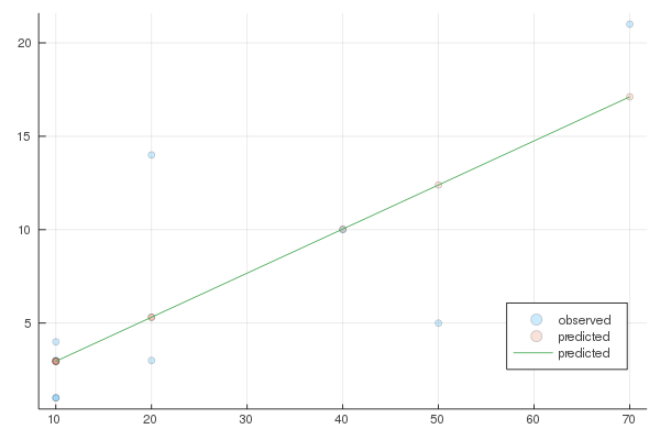
実測値と予測値の図を描いてみよう

using Plots
scatter(x, y, alpha=0.2, label="observed")
scatter!(x, predict(results), alpha=0.2, label="predicted")
x2 = minimum(x):0.1:maximum(x)
predicted = coef(results)[2] .* x2 .+ coef(results)[1]
plot!(x2, predicted, label="predicted", legend=:bottomright)

重回帰分析

ここでは，例示のためのデータセットが使われているので，まずは下記の URL から，データをダウンロードせよと言われている。
https://ai-trend.jp/wp-content/uploads/2016/07/sample-data.csv
Mac OS の場合には /Users/foo/Dwnloads/sample-data.csv にダウンロードされる。

このファイルは邪悪な Window ファイル(cp932 エンコーディング)なので（Mac OS では）普通の CSV.read() では読めない。

これを読み取るために以下のように指定する。

using DataFrames, CSV
using StringEncodings
df = CSV.File(open(read, "/Users/foo/Downloads/sample-data.csv", enc"cp932")) |> DataFrame

30 rows × 7 columns

	番号	年齢	血圧	肺活量	性別	病気	体重
	Int64	Int64	Int64	Int64	String	Int64	Int64
1	1	22	110	4300	M	1	79
2	2	23	128	4500	M	1	65
3	3	24	104	3900	F	0	53
4	4	25	112	3000	F	0	45
5	5	27	108	4800	M	0	80
6	6	28	126	3800	F	0	50
7	7	28	126	3800	F	1	43
8	8	29	104	4000	F	1	55
9	9	30	125	3600	F	1	47
10	10	31	120	3400	F	1	49
11	11	32	116	3600	M	1	64
12	12	32	124	3900	M	0	61
13	13	33	106	3100	F	0	48
14	14	33	134	2900	F	0	41
15	15	34	128	4100	M	1	70
16	16	36	128	3420	M	1	55
17	17	37	116	3800	M	1	70
18	18	37	132	4150	M	1	90
19	19	38	134	2700	F	0	39
20	20	39	116	4550	M	1	86
21	21	40	120	2900	F	1	50
22	22	42	130	3950	F	1	65
23	23	46	126	3100	M	0	58
24	24	49	140	3000	F	0	45
25	25	50	156	3400	M	1	60
26	26	53	124	3400	M	1	71
27	27	56	118	3470	M	1	62
28	28	58	144	2800	M	0	51
29	29	64	142	2500	F	1	40
30	30	65	144	2350	F	0	42

このデータファイルを使って，肺活量を血圧と体重で予測する。

指定方法は単回帰分析の場合と同じである。

using GLM
results = lm(@formula(肺活量 ~ 血圧 + 体重), df);
println(results)

StatsModels.DataFrameRegressionModel{LinearModel{LmResp{Vector{Float64}}, DensePredChol{Float64, LinearAlgebra.Cholesky{Float64, Matrix{Float64}}}}, Matrix{Float64}}

Formula: 肺活量 ~ 1 + 血圧 + 体重

Coefficients:
─────────────────────────────────────────────────────
              Estimate  Std.Error   t value  Pr(>|t|)
─────────────────────────────────────────────────────
(Intercept)  3533.07    830.819     4.25251    0.0002
血圧            -14.2164    5.57863  -2.54837    0.0168
体重             30.7853    5.09687   6.04005    <1e-05
─────────────────────────────────────────────────────

println() で表示される総括表は coeftable() で表示されるものと同じである。

coeftable(results)

─────────────────────────────────────────────────────
              Estimate  Std.Error   t value  Pr(>|t|)
─────────────────────────────────────────────────────
(Intercept)  3533.07    830.819     4.25251    0.0002
血圧            -14.2164    5.57863  -2.54837    0.0168
体重             30.7853    5.09687   6.04005    <1e-05
─────────────────────────────────────────────────────

係数だけを取り出すのは coef() である。

coef(results)

3-element Vector{Float64}:
 3533.065265426281
  -14.216447838209147
   30.785336447492494

変数名を取り出すのは coefnames() である。

coefnames(results)

3-element Vector{String}:
 "(Intercept)"
 "血圧"
 "体重"

偏回帰係数（定数項）標準誤差は stderror() である。

stderror(results)

3-element Vector{Float64}:
 830.8185624272833
   5.578634802056308
   5.096867359589727

R の summary() で出力されるもののうち，まず残差標準誤差 Residual standard error は以下のようにして求める。

残差の自由度は dof_residual(results) である。

sqrt(sum(residuals(results) .^ 2) / dof_residual(results))

368.26786392925806

dof_residual(results) # 残差の自由度

27.0

重相関係数の二乗（決定係数），および自由度調整済みの重相関係数の二乗は以下のようにして求める。

r2(results) # 重相関係数の二乗（決定係数）

0.6748009330930996

adjr2(results) # 重相関係数の二乗（決定係数）

0.6507121133222181

AIC，AICC，BIC は aic()，aicc()，bic() で求める。StatsBase が必要である。

using StatsBase
aic(results)

444.5041303923531

aicc(results)

446.1041303923531

bic(results)

450.1089199190017

そのほか，有効データ数は nobs(), 偏回帰係数の信頼区間は confint() , 自由度は dof，分散・共分散行列は vcov()，デビアンスは deviance()，対数尤度は loglikelihood()，予測値は predict()，残差は rediduals()，残差の自由度は dof_residual() で求める。

nobs(results) # 有効データ数

30.0

confint(results) # 偏回帰係数（定数項）の信頼区間

3×2 Matrix{Float64}:
 1828.37    5237.76
  -25.6629    -2.77003
   20.3274    41.2432

stderror(results) # 偏回帰係数（定数項）の標準誤差

3-element Vector{Float64}:
 830.8185624272833
   5.578634802056308
   5.096867359589727

dof(results) # モデルで消費される自由度（説明変数の個数 + 1 + 1）

vcov(results) # 偏回帰係数の分散・共分散行列

3×3 Matrix{Float64}:
     6.90259e5  -4341.97     -2496.46
 -4341.97          31.1212       7.97855
 -2496.46           7.97855     25.9781

deviance(results) # デビアンス

3.6617729292815e6

nulldeviance(results) # null モデルのデビアンス

1.126009666666667e7

loglikelihood(results) # 対数尤度

-218.25206519617655

nullloglikelihood(results) # null モデルの対数尤度

-235.10183175521513

predict(results) # 予測値

30-element Vector{Float64}:
 4401.297582575182
 3714.4068112225223
 3686.1775219696315
 3326.1632476840186
 4460.5158146990925
 3281.0596601865527
 3065.5623050541053
 3747.7481948646164
 3202.9200986822843
 3335.5730107683153
 3854.2188488335396
 3648.1312567853884
 3503.8179440557506
    ⋮
 2828.6893765584628
 4531.496250678374
 3366.358347215808
 3685.973915546104
 3527.342351766493
 2928.1027082141627
 3162.4195895152034
 3955.984621260314
 3764.215280262136
 3055.948935546281
 2745.743130300282
 2778.8809075188483

residuals(results) # 残差

30-element Vector{Float64}:
 -101.29758257518188
  785.5931887774777
  213.82247803036853
 -326.16324768401864
  339.4841853009075
  518.9403398134473
  734.4376949458947
  252.25180513538362
  397.07990131771567
   64.42698923168473
 -254.2188488335396
  251.86874321461164
 -403.81794405575056
    ⋮
 -128.68937655846275
   18.503749321625946
 -466.35834721580795
  264.02608445389615
 -427.3423517664928
   71.8972917858373
  237.58041048479663
 -555.9846212603138
 -294.2152802621358
 -255.94893554628106
 -245.7431303002818
 -428.8809075188483

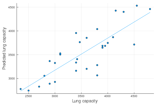
scatter(df.肺活量, predict(results), smooth=true, xlabel="Lung capacity", ylabel="Predicted lung capacity", label="")

Linear Least Square Regression の略 ↩
原点を通るモデルの場合は bias=false を指定する。 ↩

Julia 入門05 -- R と比較して（線形モデルによる回帰分析）

線形モデルによる回帰分析

llsq() 関数を用いて単回帰分析

GLM による分析

重回帰分析

`llsq()` 関数を用いて単回帰分析

`GLM` による分析