0.Prologue
暇つぶしに、興味を引いた DNNアプリを *Interpに移植して遊んでいる。
本稿はその雑記&記録。
数年前になるが、MiDaSと言う単眼視深度推定(Monoular depth estimation)モデルを Nerves/Raspberry-pi3で動かして遊んでみた。数ある単眼視深度推定モデルの中から MiDaSを選んだ理由は、ロバスト性に優れているという触れ込みだったからだ。なんでも、互換性の乏しい複数のデータセットに、ゴリゴリと工夫を凝らして学習しているそうだ。深度アノテーション付きのデータセットを作成するコストが高いため、在りもので賄おうということのようだ。どうやら深度推定では、学習に用いるデータセットを用意するところに一つ目の大きな課題があるらしい。
課題があればその解決を目指すリサーチャーがいて、"Self-Supervised Monocular Depth Prediction"なんてものが提案されている。今回は、そんなモデルの一つ SC-Depthで遊んでみようと思う。
1.Original Work
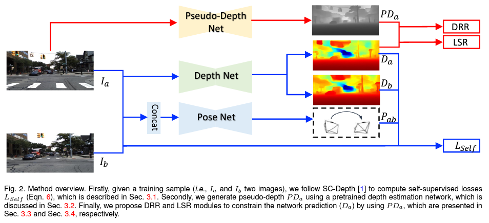
単眼視深度推定モデルを "Self-Supervised"に学習する方法は大きく二つあって、一つはステレオ視を、もう一つは単眼視エゴモーションを援用する方法のようだ。SC-Depthは後者の方法を採用している。そしてSC-Depthが特にフォーカスしているのは、(1)移動物体に対する深度推定の精度の向上と、(2)物体境界部で推定結果がぼやける課題(オクルージョンに起因する)の解決。彼らのアプローチで目を引く点は、別の学習済み単眼視深度推定モデル(LeReS)を持ってきて、その出力 -- pseudo-depthと呼んでいる -- を足場としているところかな(下図の一番上のフロー)。より詳しくは論文を参照のこと。
-
SC-DepthV3: Robust Self-supervised Monocular Depth Estimation for Dynamic Scenes
https://arxiv.org/abs/2211.03660 -
GitHub: SC_Depth
https://github.com/JiawangBian/sc_depth_pl
2.準備
SC-Depthの学習済みパラメタ(Pytorchのcheckpoint)は、下の OneDriveに置かれている。これを OnnxInterpで利用できるように ONNXモデルに変換しよう。

Pytorchのcheckpointにはモデルのグラフは含まれていないので、本家プロジェクトのモデル定義のコードが必要になる。プロジェクトをまるっと git cloneしよう。
git clone https://github.com/JiawangBian/sc_depth_pl
cd sc_depth_pl
pip install -r requirements.txt
残念ながら、本家プロジェクトには ONNXモデルをエクスポートするスクリプトは添付されていない。同梱のinference.pyを参考に、ちょこちょこっと自前で用意した。
import torch
import torch.onnx
from path import Path
import os

from config import get_opts, get_training_size

from SC_Depth import SC_Depth
from SC_DepthV2 import SC_DepthV2
from SC_DepthV3 import SC_DepthV3


@torch.no_grad()
def main():
    hparams = get_opts()

    if hparams.model_version == 'v1':
        system = SC_Depth(hparams)
    elif hparams.model_version == 'v2':
        system = SC_DepthV2(hparams)
    elif hparams.model_version == 'v3':
        system = SC_DepthV3(hparams)

    output_dir = Path(hparams.output_dir)
    output_dir.makedirs_p()

    system = system.load_from_checkpoint(hparams.ckpt_path, strict=False)

    model = system.depth_net
    model.eval()

    # training size
    training_size = get_training_size(hparams.dataset_name)
    dummy_input = torch.randn(1, 3, *training_size)

    # export the model
    torch.onnx.export(model,
        dummy_input,
        output_dir / Path(hparams.ckpt_path).stem + ".onnx",
        export_params=True,
        #opset_version=10,
        do_constant_folding=True,
        input_names=["input.0"],
        output_names=["output.0"],
        #dynamic_axes={}
        )


if __name__ == '__main__':
    main()
上の OneDriveからダウンロードした学習済みパラメタを ./ckptsディレクトリに置いたとすると、次のコマンド・ラインを実行することで ./onnx_modelディレクトリに変換されたONNXモデルが出来上がる。
!python export_onnx.py --config configs/v3/ddad.txt --output_dir onnx_model --ckpt_path ckpts/ddad_scv3/epoch\=99-val_loss\=0.1438.ckpt
このままのONNXモデルでも利用できるのだが、ONNX Simplifierでシェイプアップしておこう。
onnxsim "epoch=99-val_loss=0.1438.onnx" "sc_depth-epoch=99-val_loss=0.1438.onnx"
3.OnnxInterp用のLivebookノート
Mix.installの依存リストに記述するモジュールは下記の通り。
File.cd!(__DIR__)
# for windows JP
#System.shell("chcp 65001")

Mix.install([
  {:onnx_interp, path: ".."},
  {:cimg, "~> 0.1.18"},
  {:nx, "~> 0.4.2"},
  {:kino, "~> 0.8.0"}
])
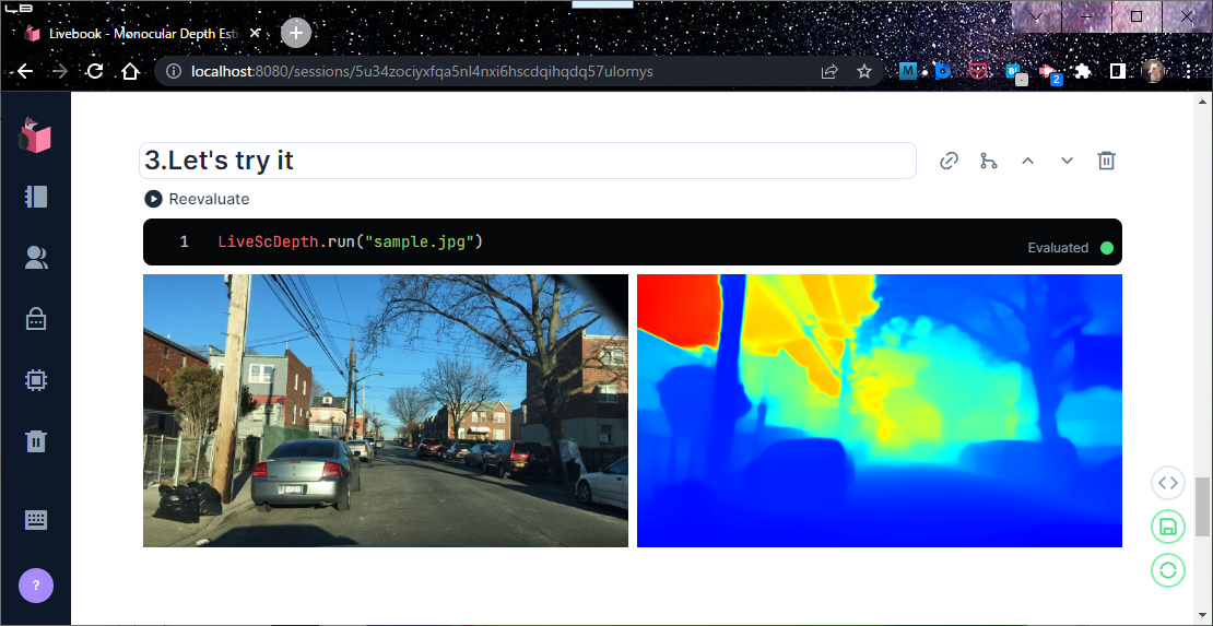
SC-Depthモデルの出力は、入力画像と同じ縦横サイズを持つ深度マップ。各行・列の要素の値は、入力画像中の対応する位置にある物体までの深度を表している。その値が大きいほど物体までの距離が遠いようだ。ただ、距離の単位やリニアリティについてはよく分からない。単なる相対値なのかなぁ? まぁなにはともあれ、この深度マップを可視化したいので、要素の値のmin-maxで正規化してグレイ画像(0..255)に変換する。さらに格好良く見せる常套手段は、ヒートマップへの変換だが、この処理はデモ・モジュールに先送る。
[モデル・カード]
- inputs:
[0] f32:{1,3,384,640} - RGB画像,NCHWレイアウト,画素は平均/分散: R{114.75,57.375},G{114.75,57.375},B{114.75,57.375}で正規化- outputs:
[0] f32:{1,1,384,640} - 入力と同じサイズの深度マップ。各要素の値は、その位置にある物体までの深度を表す。値が大きいほど距離が遠い(相対値?)。
defmodule ScDepth do
  @width  640
  @height 384

  alias OnnxInterp, as: NNInterp
  use NNInterp,
    model: "model/sc_depth-epoch=99-val_loss=0.1438.onnx",
    url: "https://github.com/shoz-f/onnx_interp/releases/download/models/sc_depth-epoch.99-val_loss.0.1438.onnx",
    inputs: [f32: {1,3,@height,@width}],
    outputs: [f32: {1,1,@height,@width}]

  def apply(img) do
    # preprocess
    input0 = CImg.builder(img)
      |> CImg.resize({@width, @height})
      |> CImg.to_binary([{:gauss, {{114.75,57.375},{114.75,57.375},{114.75,57.375}}}, :nchw])

    # prediction
    output0 = session()
      |> NNInterp.set_input_tensor(0, input0)
      |> NNInterp.invoke()
      |> NNInterp.get_output_tensor(0)

    # postprocess
    {w, h, _, _} = CImg.shape(img)

    output0
    |> CImg.from_binary(@width, @height, 1, 1, range: min_max(output0), dtype: "<f4") # Gray image
    |> CImg.resize({w,h})
  end

  defp min_max(bin) do
    t = Nx.from_binary(bin, :f32)
    {
      Nx.reduce_min(t) |> Nx.to_number(),
      Nx.reduce_max(t) |> Nx.to_number()
    }
  end
end
デモ・モジュール LiveScDepthは、ScDepthから受け取った深度マップ(グレイ画像)を色付け描画する。
defmodule LiveScDepth do
  def run(path) do
    img = CImg.load(path)

    depth = ScDepth.apply(img)
      |> CImg.color_mapping(:jet)

    Kino.Layout.grid(
      Enum.map([img, depth], &CImg.display_kino(&1, :jpeg)),
      columns: 2)
  end
end
4.デモンストレーション
ScDepthを起動する。
ScDepth.start_link([])
画像を与え、SC-Depthを実行する。
LiveScDepth.run("sample.jpg")
5.Epilogue
単眼視深度推定の SC-Depthを移植して遊んでみた。
*Interpシリーズは inferenceエンジンなので、残念ながらリサーチャーたちが SC-Depthの学習ステップに盛り込んだ工夫を体感することはできない。リソースが制限されたエッジ・デバイスで、学習なりチューニングなりを行うのはとてもハードルが高いと思うのだが、ちらほらと "On-device Training"というキーワードを見かけたりするので、少しこの方面も調べてみようかなと思う。