python のライブラリ matplotlibについて学んでいきたいと思います。
matplotlib とは
matplotlib はpythonのプロットライブラリで、散布図やヒストグラム、棒グラフをコードを使用して作成出来ます。
データ分析に使用されるもので、pip等でインストールも可能ですが、Anacondaに含まれていますので今回はそちらを使用します。
全体イメージ
今回は Jupyter Notebookを使用して実際の結果がすぐに分かるようにしました。
まず全体のイメージから理解します。
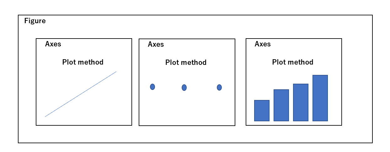
以下は基本的な散布図です。

Figure という基盤に Axes を呼ばれる枠組みを用意します。
Axesの枠組みに定義したPlotメソッドを使用して図を描いていきます。
これがmatplotlibの基本的な描き方かと思います。
先ほどJupyter Notebookから実行したコードに注釈を入れると、以下のようなイメージになります。
# matplotlib のインポート
import matplotlib.pyplot as plt

# プロットする点の定義
X = [1,2,3]
Y = [1,1,1]

# figureオブジェクトを生成する
fig = plt.figure()

# axesオブジェクトをfigureオブジェクトに対して設定する
ax = fig.add_subplot(1, 1, 1)

# axesオブジェクトに対して散布図のメソッドを設定する
ax.scatter(X, Y)

# 表示させる
plt.show()
Figure について
グラフィックの基盤となるものを定義します。
引数は公式に記載がありますが、全体のフレームをどのようにしたいかを定義するものとなるかと思います。
先ほど plt.figure()へ定義したものに、少し手を加えてみます。
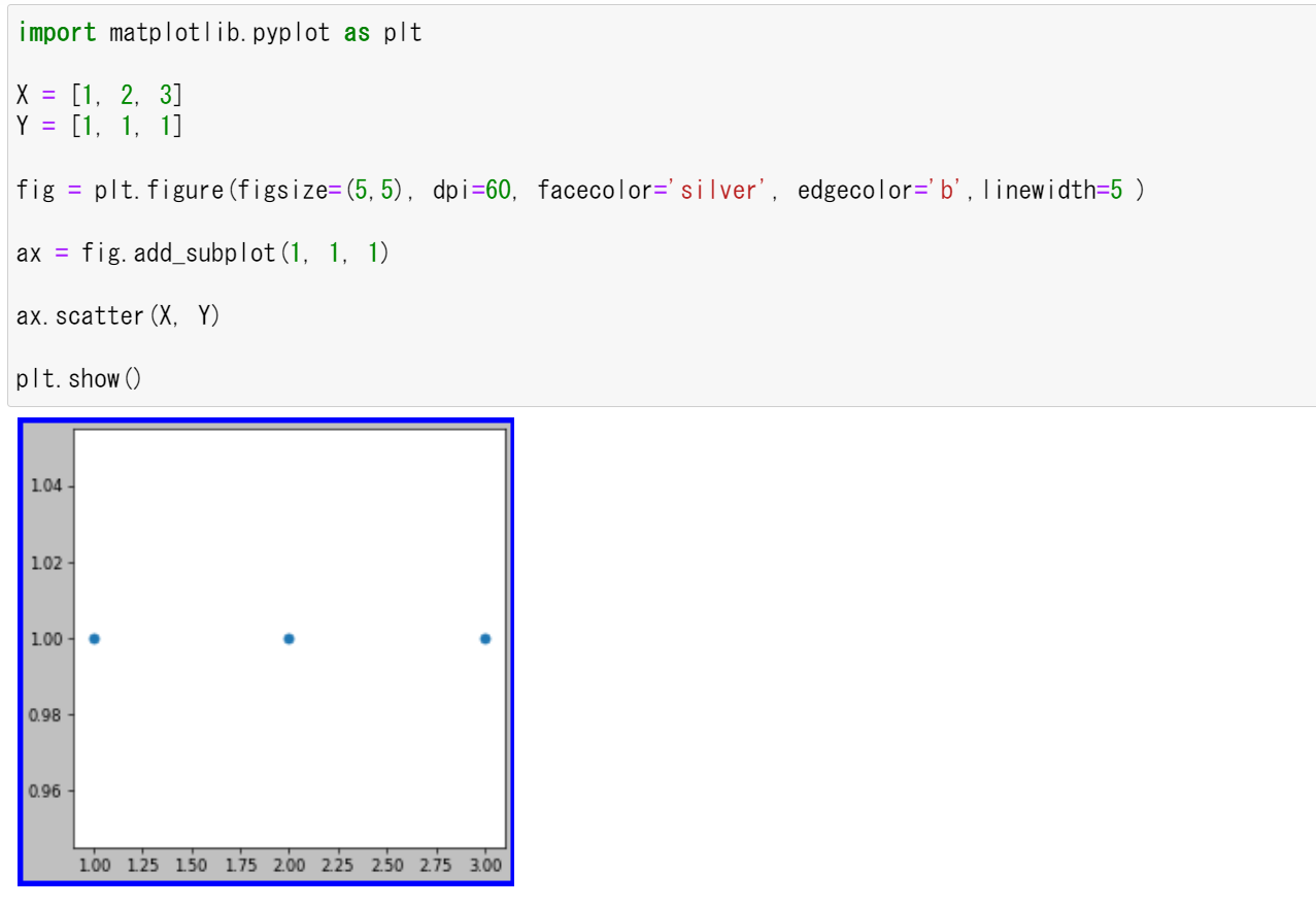
fig = plt.figure(figsize=(5,5), dpi=60, facecolor='silver', edgecolor='b',linewidth=5)
| Property | Description |
|---|---|
| figsize | 枠組みのサイズ、float値で(width, height)を指定 |
| dpi | 解像度を整数で指定 |
| facecolor | 背景色を指定、16 進数のカラーコードも指定可 |
| edgecolor | 枠の色を指定、b は "Blue"の省略 |
| linewidth | 枠線の太さを指定、整数 |
Axes について
Figure の上に作成される枠組みであり、この中にグラフが描かれます。
Axes は複数作成することができます。一般的に、グラフの種類に応じたメソッドに対して、リストやndarrayなどのシーケンスを引数に設定します。
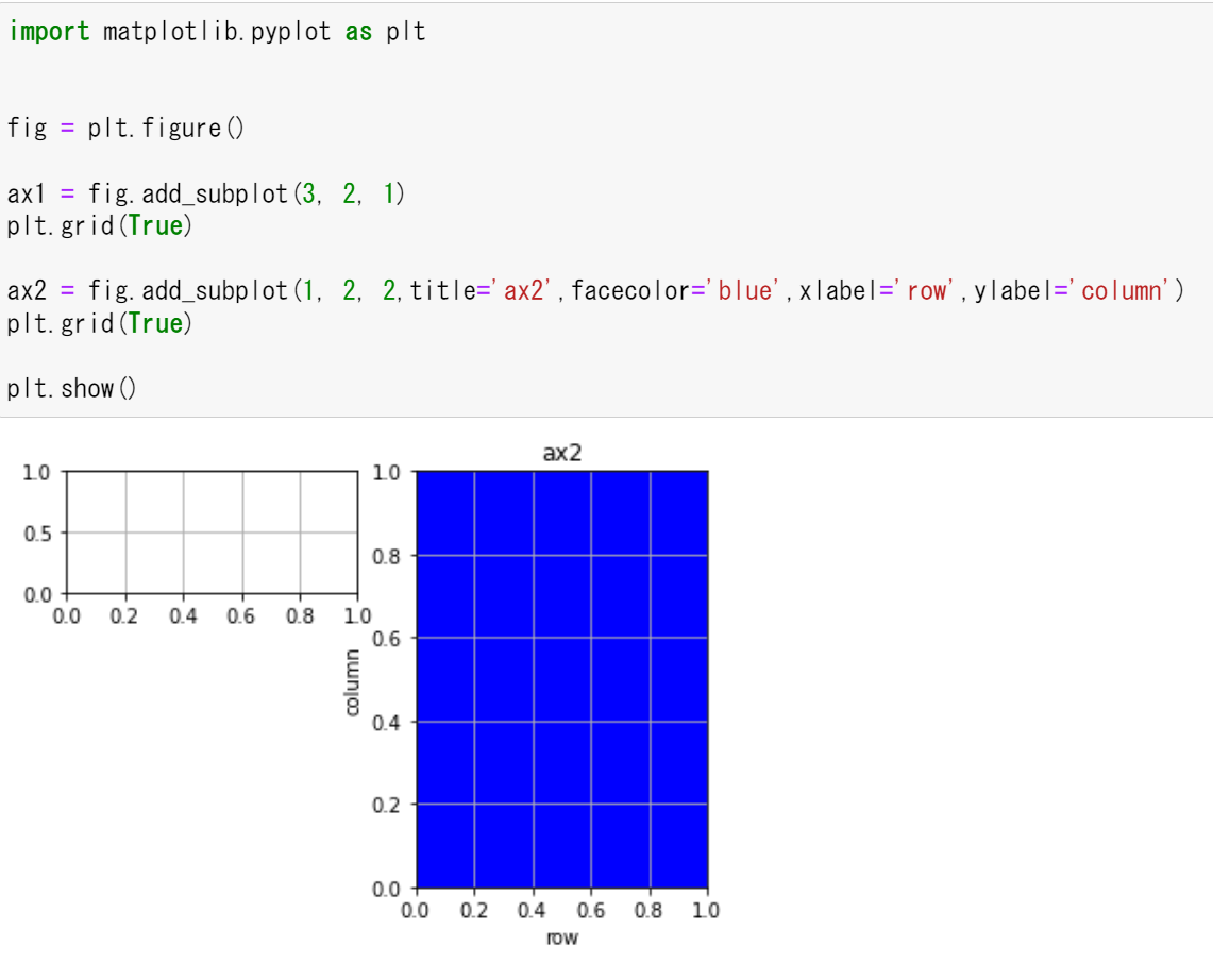
add_subplot()
以下の例では、add_subplot()メソッドを使用して複数のaxesを定義しています。

import matplotlib.pyplot as plt

fig = plt.figure()

# 1つ目のaxesオブジェクトをfigureオブジェクトに対して設定する
ax1 = fig.add_subplot(2, 3, 1)
# 2つ目のaxesオブジェクトをfigureオブジェクトに対して設定する
ax2 = fig.add_subplot(2, 3, 2)
# 3つ目のaxesオブジェクトをfigureオブジェクトに対して設定する
ax3 = fig.add_subplot(2, 3, 3)
# 4つ目のaxesオブジェクトをfigureオブジェクトに対して設定する
ax4 = fig.add_subplot(2, 3, 4)

plt.show()
add_subplot() は (nrows, ncols, index)を入れます。
Figureを行としてnrows分割、列としてncols分割したうち、indexの位置にAxesが返されます。
他にもpropertyを指定する事で、表示形式を変更出来ます。

| Property | Description |
|---|---|
| title | 文字列のタイトルを指定 |
| facecolor | axesの色を指定 |
| xlabel | X軸のタイトルを指定 |
| ylabel | Y軸のタイトルを指定 |
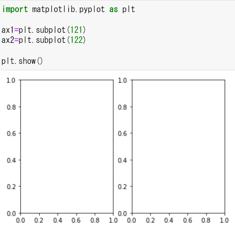
plt.subplot( )
add_subplot() メソッドは、Figureオブジェクト上に定義しますが、
plt.subplot() メソッドは、Figureオブジェクトの生成が不要となります。
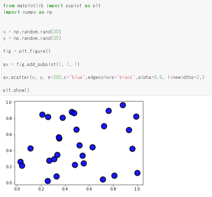
散布図 ax.scatter
散布図を描くには ax.scatter()メソッドを使用します。
以下の例では、Numpyライブラリの np.random.randを使用して乱数を生成して点を生成しています。
from matplotlib import pyplot as plt
import numpy as np

# 乱数を生成
x = np.random.rand(30)
y = np.random.rand(30)

# figureを生成
fig = plt.figure()

# axをfigureに設定
ax = fig.add_subplot(1, 1, 1)

# 散布図を生成
ax.scatter(x, y, s=200,c='blue',edgecolors='black',alpha=0.9, linewidths=2,)

#表示
plt.show()
| Property | Description |
|---|---|
| x | X座標データ配列 |
| y | Y座標データ配列 |
| s | マーカーのサイズ |
| c | マーカーの色 |
| marker | マーカーの形(デフォルトはo) |
| alpha | マーカーの透明度 |
| linewidths | マーカーの枠のサイズ |
| edgecolors | マーカーの枠の色 |
棒グラフ ax.bar
棒グラフを描くには ax.bar()メソッドを使用します。
以下の例では x,height,Labelに定義した配列をax.barで使用します。

import matplotlib.pyplot as plt

# 縦軸、横軸のデータ
x = [1, 2, 3, 4, 5, 6]
height = [2, 3, 2, 2, 5, 4]

# ラベル
label = ['A', 'B', 'C', 'D', 'E', 'F']

# figureを生成
fig = plt.figure()

# axをfigureに設定
ax = fig.add_subplot(1, 1, 1)

# axesに棒グラフを設定
ax.bar(x, height, trick_label=label,edgecolor="Blue")

# 表示
plt.show()
| Property | Description |
|---|---|
| x | X座標データ配列 |
| height | 棒の高さのデータ配列 |
| trick_label | 棒単位の名称 |
| color | 棒の色 |
| edgecolor | 棒の枠の色 |
円グラフ ax.pie
円グラフを描くには、ax.pieメソッドを使用します。
以下の例では、label,xに定義した配列をax.pieで使用します。
また、ax.axisは表示補正のために呼び出しを行うようです。

import matplotlib.pyplot as plt

# 対象データ
label = ["A", "B", "C", "D", "E", "F"]
x = [20, 10, 36, 20, 2, 12]

# figureを生成
fig = plt.figure()

# axをfigureに設定
ax = fig.add_subplot(1, 1, 1)

# ax に円グラフを設定
ax.pie(x, labels=label, counterclock=False, startangle=90)

# 表示補正
ax.axis('equal')

# 表示
plt.show()
| Property | Description |
|---|---|
| x | データ配列 |
| labels | 各要素のラベルの配列 |
| counterclock | 時計周り(False),反時計周り(True) |
| startangle | 開始角度(デフォルトは3時から開始) |
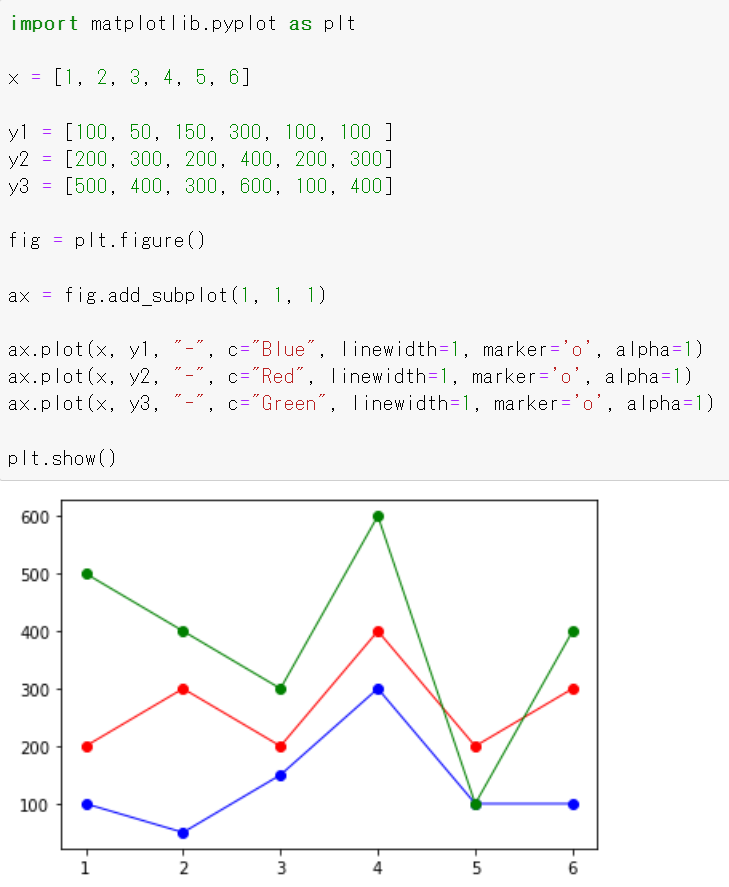
折れ線グラフ ax.plot
折れ線グラフは、ax.plotメソッドを使用します。
以下の例では、x 軸に6つのデータを定義し、折れ線となる軸を3つ、かつy軸の線に対する値を6つ定義します。
import matplotlib.pyplot as plt

# X軸の定義
x = [1, 2, 3, 4, 5, 6]

# Y軸の定義
y1 = [100, 50, 150, 300, 100, 100 ]
y2 = [200, 300, 200, 400, 200, 300]
y3 = [500, 400, 300, 600, 100, 400]

# figureを生成
fig = plt.figure()

# axをfigureに設定
ax = fig.add_subplot(1, 1, 1)

# axに折れ線を設定
ax.plot(x, y1, "-", c="Blue", linewidth=1, marker='o', alpha=1)
ax.plot(x, y2, "-", c="Red", linewidth=1, marker='o', alpha=1)
ax.plot(x, y3, "-", c="Green", linewidth=1, marker='o', alpha=1)

# 表示
plt.show()
| Property | Description |
|---|---|
| x | X座標配列データ |
| y | Y座標配列データ |
| c | 折れ線の色 |
| linewidth | 折れ線の太さ |
| marker | X軸のデータに到達した際の点の形(デフォルトはo) |
| alpha | 線の透明度 |
その他汎用要素
plt.grid() は、グリッド線を追加する事が出来ます。
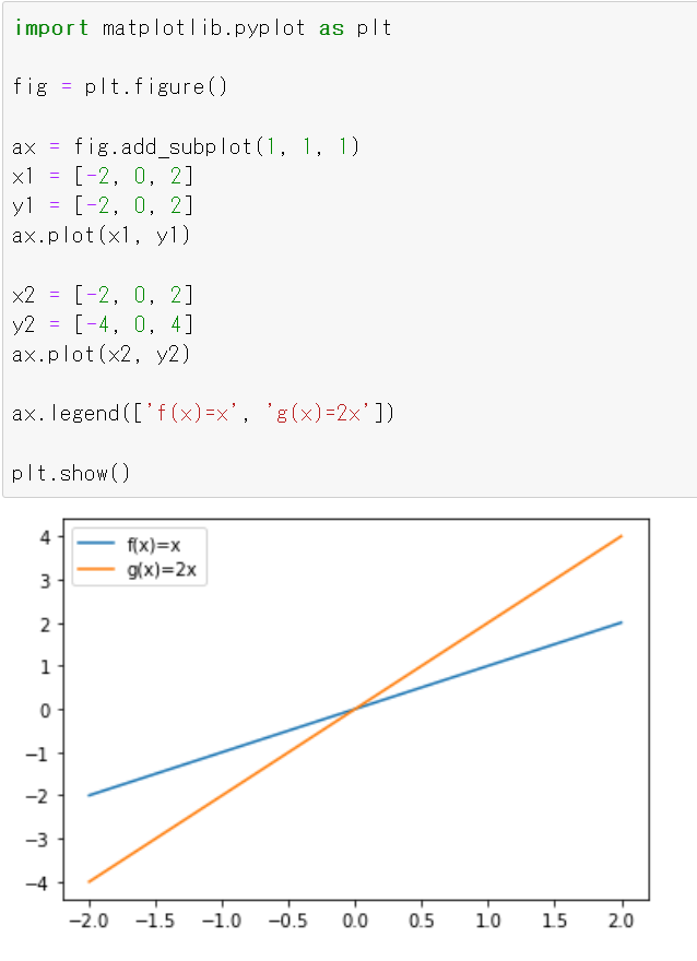
ax.legend() は、凡例を表示するものです。
グラフを描画したものに対して補足説明をする際に、使用します。
使用してみると、可視化されるので非常に面白かったです。
以上です。