本記事では、pycprops (pythonでCPROPSを使うモジュール) の使い方について紹介します。
まず pycprops をインストールします。
pip install pycprops
うまくいかない場合はドキュメントをしっかり読むか、エラーメッセージで google 検索して対処しましょう。
今回、適用データとして scimes に同梱されていた orion_12CO.fits (3D) と orion_12CO_mom0.fits (2D) を用います。
3D の場合
必要なものを import します。
import pycprops
import astropy.units as u
from astropy.io import fits
import numpy as np
import aplpy
import matplotlib.pyplot as plt
ドキュメント通りに以下を実行します。先に言っておくと、ヘッダの CTYPE3 を VELOCITY にして、さらに RESTFREQ が書かれていないとエラーが起こります。
cubefile = "orion_12CO.fits"  # Your cube
mask = "orion_12CO.fits" # Mask defining where to find emission
d = 420.0 * u.pc           # Distance (with units)

# ValueError: No spectral axes found in WCS
エラーが出ました。fits のヘッダを確認します。
fits.getheader(cubefile)
# SIMPLE  =                    T / Written by IDL:  Fri Sep 23 12:30:50 2005
# BITPIX  =                  -32 / IEEE single precision floating point
# NAXIS   =                    3 /number of axes
# NAXIS1  =                  209 /
# NAXIS2  =                  177 /
# NAXIS3  =                  150 /
# EXTEND  =                    T /file may contain extensions
# BSCALE  =              1.00000 /  REAL = TAPE*BSCALE + BZERO
# BZERO   =              0.00000 /
# BUNIT   = 'K                 ' /  UNIT OF TOTAL INTENSITY
# BLANK   =               -32768 / BLANK VALUE
# OBJECT  = 'Orion             ' /  SOURCE NAME
# CRVAL1  =        226.000000000 / REF VALUE POINT DEGREE
# CRPIX1  =        1.00000000000 / REF POINT PIXEL LOCATION
# CTYPE1  = 'GLON-CAR          ' / COORD TYPE : VALUE IS DEGR
# CDELT1  =      -0.125000000000 / COORD VALUE INCREMENT WITH KM/S
# CROTA1  =       0.000000000000 / NO ROTATION
# CRVAL2  =       -25.0000000000 / REF VALUE POINT DEGREE
# CRPIX2  =        1.00000000000 / REF POINT PIXEL LOCATION
# CTYPE2  = 'GLAT-CAR          ' / COORD TYPE : VALUE IS DEGR
# CDELT2  =       0.125000000000 / COORD VALUE INCREMENT WITH COUNT DGR
# CROTA2  =       0.000000000000 / NO ROTATION
# CRVAL3  =        46485.9924316 / REF VALUE POINT DEGREE
# CRPIX3  =        1.00000000000 / REF POINT PIXEL LOCATION
# CTYPE3  = 'M/S     '           / COORD TYPE : VALUE IS DEGR
# CDELT3  =       -650.153696537 / COORD VALUE INCREMENT WITH COUNT DGR
# CROTA3  =       0.000000000000 / NO ROTATION
# TELESCOP= '1.2m              ' /
# O_BSCALE=          0.000746469 / Original BSCALE Value
# O_BZERO =              6.91305 / Original BZERO Value
# BMAJ    =             0.133333 /
# BMIN    =             0.133333 /
3軸目が spectral だと認識していないようですので、以下のように書き換えます。
hdu = fits.open(cubefile)[0]
d, h = hdu.data, hdu.header
h["CTYPE3"] = "VELOCITY"
fits.PrimaryHDU(d, h).writeto(cubefile[:-5]+".header_change.fits", overwrite=True)
仕切り直してもう一回実行します。
cubefile = "orion_12CO.header_change.fits"  # Your cube
mask = "orion_12CO.header_change.fits" # Mask defining where to find emission
d = 420.0 * u.pc           # Distance (with units)

pycprops.fits2props(cubefile,
                    mask_file=mask,
                    distance=d,
                    asgnname=cubefile[:-5]+".asgn.fits",
                    propsname=cubefile[:-5]+".props.fits")

# ValueError: If converting from speed to wavelength/frequency, a reference wavelength/frequency is required.
長いプロセスの後にこれを言われました。RESTFREQ をヘッダに入れて仕切り直します。
hdu = fits.open(cubefile)[0]
d, h = hdu.data, hdu.header
h["RESTFREQ"] = 115271202000.0
fits.PrimaryHDU(d, h).writeto(cubefile[:-5]+".freq.fits", overwrite=True)

cubefile = "orion_12CO.header_change.freq.fits"  # Your cube
mask = "orion_12CO.header_change.freq.fits" # Mask defining where to find emission
d = 420.0 * u.pc           # Distance (with units)

pycprops.fits2props(cubefile,
                    mask_file=mask,
                    distance=d,
                    asgnname=cubefile[:-5]+".asgn.fits",
                    propsname=cubefile[:-5]+".props.fits")
# !!!異常に時間がかかります!!!
orion_12CO.header_change.freq.asgn.fits という名前で ID の cube が出力されます。astropy.io.fits で開いて、以下を参考にしながら自由に解析しましょう。
天文データ解析入門 その20 (pycupid: pythonでclumpfind等を使う)
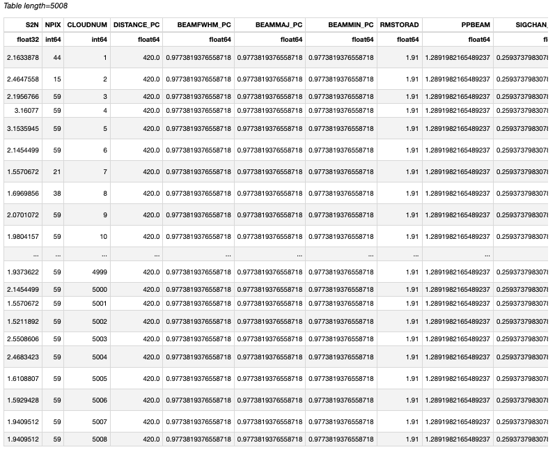
テーブルは orion_12CO.header_change.freq.props.fits という名前で出力されます。
このファイルは以下のように開きます。
from astropy.table import Table
props = Table(fits.open(cubefile[:-5]+".props.fits")[1].data)
props
pandas 形式で使いたい方は、以下のようにします。
import pandas as pd
df = props.to_pandas()
2D の場合
結論から言うと、2D fits には対応していません。なので、無理やり cube にして実行します。
必要なものを import します。
import pycprops
import astropy.units as u
from astropy.io import fits
import numpy as np
import aplpy
import matplotlib.pyplot as plt
fitsname = "orion_12CO_mom0.fits"
hdu_2D = fits.open(fitsname)[0]

d = hdu_2D.data.reshape(1, hdu_2D.data.shape[0], hdu_2D.data.shape[1])
d_ = np.zeros_like(d)
d_[d_==0] = np.nan
d = np.concatenate([d, d_], axis=0)
h = hdu_2D.header

h["NAXIS"] = 3
h["NAXIS3"] = 2
h["CDELT3"] = 1
h["CRVAL3"] = 1
h["CRPIX3"] = 1
h["CTYPE3"] = "VELOCITY"
h["RESTFREQ"] = 115271202000.0
h["BUNIT"] = "K"

fits.PrimaryHDU(d, h).writeto(fitsname[:-5]+".fake3D.fits", overwrite=True)
orion_12CO_mom0.fake3D.fits を作りました。 0ch目にデータが入っており、1ch目には全部 NaN が入っています。
cubefile = "orion_12CO_mom0.fake3D.fits"  # Your cube
mask = cubefile # Mask defining where to find emission
d = 420.0 * u.pc           # Distance (with units)

pycprops.fits2props(cubefile,
                    mask_file=mask,
                    distance=d,
                    asgnname=cubefile[:-5]+".asgn.fits",
                    propsname=cubefile[:-5]+".props.fits")
# これは現実的な時間で終わります。
結果を plot してみます。
fig = plt.figure(figsize=(8, 8))
f = aplpy.FITSFigure(cubefile[:-5]+".asgn.fits", slices=[0],convention='wells', figure=fig)
f.show_colorscale(cmap="jet", aspect="equal")
f.add_colorbar()
f.colorbar.show()
plt.show()
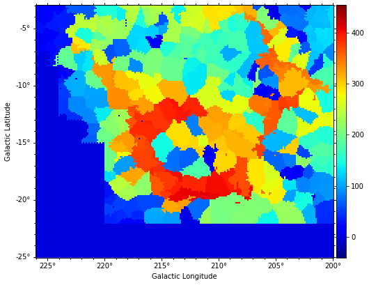
カラーが cloud の ID を示しています。
出力されたテーブル (fits 形式) を見てみます。
from astropy.table import Table
props = Table(fits.open(cubefile[:-5]+".props.fits")[1].data)
props

pandas 形式で使いたい方は、以下のようにします。
import pandas as pd
df = props.to_pandas()
ここまで来ればあとは自由に解析できます。
同定パラメータについて
残念ながら pycprops のページには一切何も書かれていません。一応、pycprops.fits2props の引数としては以下のようになっています。
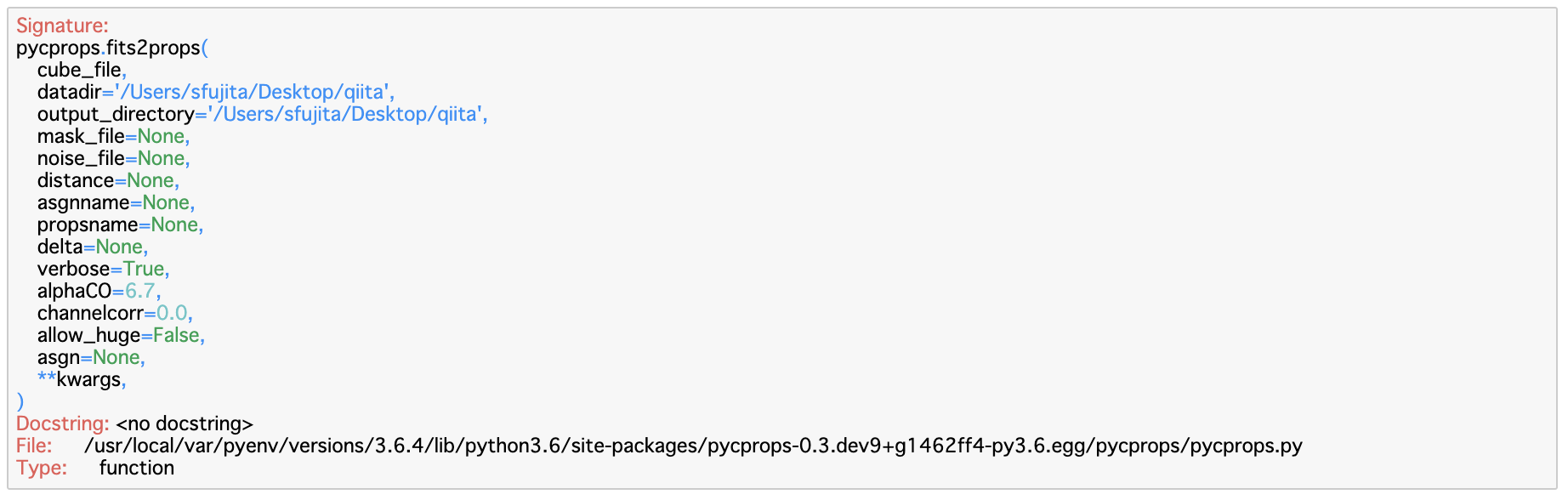
公式のページ を読むか、コードを見れば何かわかるかもしれません。
以上です。
リンク
目次