雑にsimulated annealingする話

この記事はIQ1AdcC2019(2枚目)の5日目の記事です。
（書き忘れてた。@chakku_000すまん）

磁性体の単純なモデルとして、Ising模型とかPotts模型とかXY模型とか呼ばれるものがある。

こいつらの基底状態を雑なsimulated annealingで求めてみる。

simulated annealing とは

焼きなまし法（やきなましほう、英: Simulated Annealing、SAと略記、疑似アニーリング法、擬似焼きなまし法、シミュレーティド・アニーリングともいう）は、大域的最適化問題への汎用の乱択アルゴリズムである。広大な探索空間内の与えられた関数の大域的最適解に対して、よい近似を与える。
(Wikipediaより)

雑に言ってしまえば最適化問題を解くためのヒューリスティックな手法の1つだ。
基本的には勾配を下るのだが、温度$T$というパラメータを導入し確率的に山を登ることがある。
初期条件によっては局所解にはまってしまう勾配降下法とは違い、たまに山を登ることで大域最適解を見つけるアルゴリズムである。
温度はイテレーションを繰り返すたびに少しずつ小さくしていく。
この温度の制御をうまくやってあげると大域最適解が見つかる確率が1に近くなる。
（しかし大抵の場合収束がかなり遅いので、途中で打ち切って近似解を求めることが多い）

アルゴリズムは
1. $t$ 番目の状態 $\vec{s}_{t}$ の近傍からある状態$\vec{p}$ を選ぶ。
2. $E(\vec{p}) < E(\vec{s}_t)$ であれば $\vec{s}_{t+1} = \vec{p}$ に遷移。 （エネルギーが小さければ必ず遷移する）
3. $E(\vec{p}) > E(\vec{s}_t)$ であれば、確率 $e^{ (E(\vec{s}_t)-E(\vec{p}))/T }$ で $\vec{s}_{t+1}=\vec{p}$ に遷移。（エネルギーが大きければ確率で遷移）
4. 温度 $T$ を少し小さくする。
というのを適当な回数繰り返してあげるだけである。
ここで、$E$ はその状態のエネルギーである。

$T$ が十分大きいとエネルギーが大きい方に遷移する確率も大きくなるが、
$T$ が0に近くにつれてほぼ勾配降下法と同じように解を探索するようになる。

各モデルの基底クラス & SA を行うクラスStatModel を実装する。
役割でクラスを分けろ？ 知らん

import numpy as np
import matplotlib.pyplot as plt
from abc import *
import time

class StatModel (ABC):

    def __init__ (self, N, J, h):
        self.N = N;
        self.J = J;
        self.h = h;

    @abstractmethod
    def hamiltonian (self, state):
        raise NotImplementedError()

    @abstractmethod
    def update (self, state):
        raise NotImplementedError()

    @abstractmethod
    def initializeState (self):
        raise NotImplementedError()

    def prob (self, current, proposal, temperature):
        tmp = np.exp ((current-proposal)/temperature)
        return min ([tmp,1.])

    def scheduleLogarithm (self, step, beta0=1.0):
        return 1/ (beta0 * np.log (2+step))


    def annealing (self, maxStep, Tinit=1e3, C=0.995, seed=24):
        '''
        雑にSAする
        '''
        np.random.seed (seed)
        t = Tinit
        hams = []
        ts = []
        state = self.initializeState ()
        startTime = time.time ()
        times = []

        for step in range (maxStep):
            ham = self.hamiltonian (state)
            hams.append (ham)
            times.append (time.time()-startTime)
            proposal = self.update (state.copy ())
            hamprop = self.hamiltonian (proposal)
            if (np.random.rand () < self.prob (ham,hamprop,t)):
                state = proposal;

            t *= C    # 温度を下げる


        hams.append (ham);
        times.append (time.time()-startTime)
        return state, hams, times;

SA の最適な温度制御はlogの逆数なのだが、前述の通り遅い。
なので温度は指数で減らしていく。
抽象メソッドhamiltonian はエネルギーを計算するメソッドを具体的なモデルに合わせて実装する。
update メソッドは次の状態の候補を作成する。
initializeState メソッドは探索の初期状態を与える。
prob は遷移確率を求める。
annealing はMetropolis-Hastings algorithm とかいうのを使って状態遷移しつつ焼きなましする。

Ising 模型

Ising 模型はエネルギーが以下で与えられる。

E (s_1, s_2, \dots, s_N) = - \cfrac{1}{2} \sum_{i=1}^N \sum_{j=1}^N J_{ij} s_i s_j

ここで、$s_i$ は $\pm1$ の 2値をとる。
$J_{ij}$ は結合荷重である。
特に自己結合 $J_{ii}=0$ とする。
$J_{ij}$ に関しては以下の模型も同様である。
（本当は外場とか呼ばれる奴もいるんだが面倒なので無視）

class IsingModel (StatModel):

    def __init__ (self, N, J, h):
        super().__init__ (N, J, h.reshape ((N,)));

    # override
    def hamiltonian (self, state):
        tmp1 = -0.5 * state.reshape((1,self.N)) @ self.J @ state.reshape((self.N,1))
        tmp2 = -state.reshape ((1,self.N)) @ self.h
        return (tmp1 + tmp2)[0,0]

    # override
    def update (self, state):
        idx = np.random.randint (low=0,high=self.N)
        state[idx] = - state[idx]    # flip
        return state

    # override
    def initializeState (self):
        return np.sign (np.random.randn (self.N,))

li = 32
Ni = li*li
Ji = np.ones ((Ni,Ni)) - np.eye (Ni)
hi = np.zeros ((Ni,1))
maxStepi = 10000

modeli = IsingModel (Ni,Ji,hi)
statei, hamsi, timesi = modeli.annealing (maxStepi)

plt.figure ()
plt.plot (timesi, hamsi)
plt.xlabel ('times [sec]')
plt.ylabel ('energy')
plt.figure ()
plt.imshow (statei.reshape (li,li))

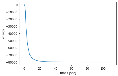
全結合強磁性モデル(全ての$i,j (i \neq j)$ で $J_{ij}=1$) を考える。
全部同じ値をとれば焼きなまし成功。

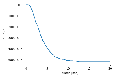
エネルギーは順調に下がっていってる。

全部同じ値なのでうまく行ったっぽい。

Potts 模型

Potts 模型のエネルギーは以下で与えられる。

E (\theta_1, \theta_2, \dots, \theta_N)
= - \cfrac{1}{2} \sum_{i=1}^N \sum_{j=1}^N J_{ij} \cos (\theta_i - \theta_j)

ここで$\theta_i$ は $2\pi n/q (n=1,2,\dots,q)$ の$q$ 値をとる。
特に$q=2$ の時はIsing 模型と完全に一致する。

class PottsModel (StatModel):

    def __init__ (self, N, J, h, q):
        super ().__init__ (N, J, h.reshape((N,)))
        self.q = q

    # override
    def hamiltonian (self, state):
        # 位相表記に変える
        phase = 2*np.pi*state/self.q
        rv = phase.reshape ((1,self.N))
        cv = phase.reshape ((self.N,1))
        tmp1 = self.J * np.cos (cv-rv)
        tmp2 = self.h @ phase.reshape (self.N,)
        return -0.5 * tmp1.sum () - tmp2

    # override
    def update (self, state):
        idx = np.random.randint (low=0, high=self.N)
        state[idx] = np.random.randint (low=0, high=self.q)
        return state

    #override
    def initializeState (self):
        return np.random.randint (low=0, high=self.q, size=(self.N,))

lp = 20
Np = lp*lp
Jp = np.ones ((Np,Np))
hp = np.zeros ((Np,))
q=4
maxStepp = 10000


modelp = PottsModel (Np, Jp, hp, q=q)
statep, hamsp, timep = modelp.annealing (maxStepp)

plt.figure ()
plt.plot (timep, hamsp)
plt.xlabel ('times [sec]')
plt.ylabel ('energy')
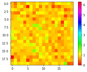
plt.figure ()
im = plt.imshow (statep.reshape (lp,lp), vmin=0, vmax=q-1)
plt.colorbar (im)

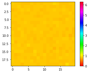
Ising 模型と同じく全結合強磁性モデル。

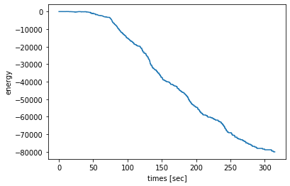
エネルギーは減り続けている。

全部同じ値なのでこれも焼きなまし成功っぽい。
エネルギーが下がりきっているようには見えないが、もうちょっと時間があれば平らになりそう。

XY 模型

XY 模型のエネルギーは以下で与えられる。

E (\mathbf{s}_1, \mathbf{s}_2, \dots, \mathbf{s}_N)
= - \cfrac{1}{2} \sum_{i=1}^N \sum_{j=1}^N J_{ij} \mathbf{s}_i \cdot \mathbf{s}_j

ここで$\mathbf{s}_i$ は2次元単位ベクトル。
Potts模型で$q\rightarrow\infty$ としたのがXY模型である。

class XYModel (StatModel):

    def __init__ (self, N, J, h):
        '''
        h は2次元列ベクトルの外場
        '''
        super().__init__ (N, J, h.reshape ((2,N)))

    # override
    def hamiltonian (self, state):
        '''
        state は2次元単位列ベクトルがN個
        '''
        tmp1 = -0.5 * self.J * (state.T @ state)
        tmp2 = - self.h * state
        return tmp1.sum() + tmp2.sum()

    #override
    def update (self, state):
        idx = np.random.randint (low=0, high=self.N)
        tmp = 2*np.pi*np.random.rand ()
        state[0,idx] = np.cos (tmp)
        state[1,idx] = np.sin (tmp)
        #print (np.arctan2 (state[1,idx], state[0,idx]))
        return state

    # override
    def initializeState (self):
        tmp = 2*np.pi*np.random.rand (1,self.N)
        return np.r_[np.cos (tmp), np.sin (tmp)]

import matplotlib.cm as cm

lx = 20
Nx = lx*lx
Jx = np.ones ((Nx,Nx))
hx = np.zeros ((2, Nx))
maxStepx = 10000



modelx = XYModel (Nx, Jx, hx)
statex, hamsx, timesx = modelx.annealing (maxStepx)

plt.figure ()
plt.plot (timesx, hamsx)
plt.xlabel ('times [sec]')
plt.ylabel ('energy')
plt.figure ()
im = plt.imshow (np.arctan2 (statex[1,:],statex[0,:]).reshape (lx,lx), cmap=cm.hsv, vmin=0, vmax=2*np.pi)
plt.colorbar(im)

これも全結合強磁性モデル。

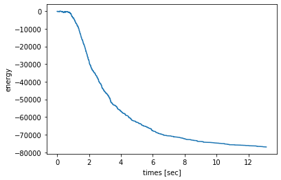
エネルギーはまだ下がりそう。

だいたい同じ色だけど、もうちょっとうまくいける気がする。

ステップ数を10倍にして見ると


まあ結構いい感じかな。
（連続値なので満遍なく全部同じ値はほぼ不可能）

まとめ

雑にSAした。
Ising 模型もXY模型もまあいい感じなんだが、Pottsだけめちゃくちゃ遅い。
多分もっと速くやる方法がある気がする。