OpenCV4.0.0のサンプルをやってみました(途中)
開発環境
Windows 10
Anaconda 4.5.11
Python 3.6.5
OpenCV 4.0.0.21
インストール
Anacondaを入れて、pipする
pip install opencv-python
pip install opencv-contrib-python
参考まで
PythonでOpenCVをはじめる(Windows10、Anaconda 2018.12、Python3.7.1、OpenCV4.0.0)
python\asift.py
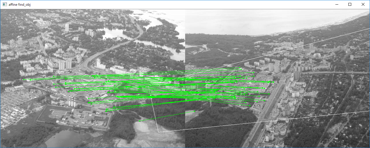
(py36) D:\python-opencv-sample>python asift.py

Affine invariant feature-based image matching sample.

This sample is similar to find_obj.py, but uses the affine transformation
space sampling technique, called ASIFT [1]. While the original implementation
is based on SIFT, you can try to use SURF or ORB detectors instead. Homography RANSAC
is used to reject outliers. Threading is used for faster affine sampling.

[1] http://www.ipol.im/pub/algo/my_affine_sift/

USAGE
  asift.py [--feature=<sift|surf|orb|brisk>[-flann]] [ <image1> <image2> ]

  --feature  - Feature to use. Can be sift, surf, orb or brisk. Append '-flann'
               to feature name to use Flann-based matcher instead bruteforce.

  Press left mouse button on a feature point to see its matching point.

using brisk-flann
affine sampling: 43 / 43
affine sampling: 43 / 43
img1 - 39500 features, img2 - 24714 features
matching ...
3545.36 ms
59 / 125  inliers/matched
Done
python\browse.py
(py36) D:\python-opencv-sample>python browse.py

browse.py
=========

Sample shows how to implement a simple hi resolution image navigation

Usage
-----
browse.py [image filename]


generating 4096x4096 procedural image ...
Done
python\calibrate.py
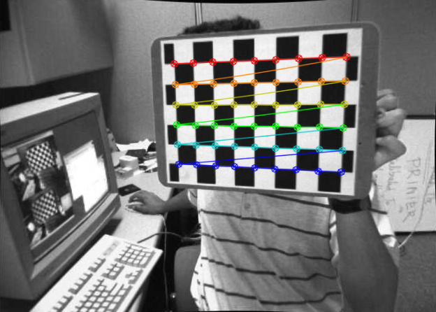
(py36) D:\python-opencv-sample>python calibrate.py

camera calibration for distorted images with chess board samples
reads distorted images, calculates the calibration and write undistorted images

usage:
    calibrate.py [--debug <output path>] [--square_size] [<image mask>]

default values:
    --debug:    ./output/
    --square_size: 1.0
    <image mask> defaults to ../data/left*.jpg

Run with 4 threads...
processing ./data\left01.jpg...
processing ./data\left02.jpg...
processing ./data\left04.jpg...
processing ./data\left03.jpg...
           ./data\left04.jpg... OK
processing ./data\left05.jpg...
           ./data\left03.jpg... OK
           ./data\left02.jpg... OK
processing ./data\left06.jpg...
processing ./data\left07.jpg...
           ./data\left01.jpg... OK
processing ./data\left08.jpg...
           ./data\left05.jpg... OK
processing ./data\left09.jpg...
           ./data\left07.jpg... OK
processing ./data\left11.jpg...
           ./data\left08.jpg... OK
processing ./data\left12.jpg...
           ./data\left06.jpg... OK
processing ./data\left13.jpg...
           ./data\left12.jpg... OK
processing ./data\left14.jpg...
           ./data\left09.jpg... OK
           ./data\left13.jpg... OK
           ./data\left11.jpg... OK
           ./data\left14.jpg... OK

RMS: 0.19643790890334015
camera matrix:
 [[532.79536562   0.         342.45825163]
 [  0.         532.91928338 233.90060514]
 [  0.           0.           1.        ]]
distortion coefficients:  [-2.81086258e-01  2.72581010e-02  1.21665908e-03 -1.34204274e-04
  1.58514023e-01]

Undistorted image written to: ./output/left01_undistorted.png
Undistorted image written to: ./output/left02_undistorted.png
Undistorted image written to: ./output/left03_undistorted.png
Undistorted image written to: ./output/left04_undistorted.png
Undistorted image written to: ./output/left05_undistorted.png
Undistorted image written to: ./output/left06_undistorted.png
Undistorted image written to: ./output/left07_undistorted.png
Undistorted image written to: ./output/left08_undistorted.png
Undistorted image written to: ./output/left09_undistorted.png
Undistorted image written to: ./output/left11_undistorted.png
Undistorted image written to: ./output/left12_undistorted.png
Undistorted image written to: ./output/left13_undistorted.png
Undistorted image written to: ./output/left14_undistorted.png
Done
python\camera_calibration_show_extrinsics.py
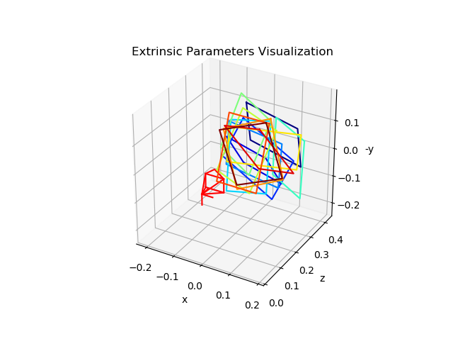
(py36) D:\python-opencv-sample>python camera_calibration_show_extrinsics.py
None
Done
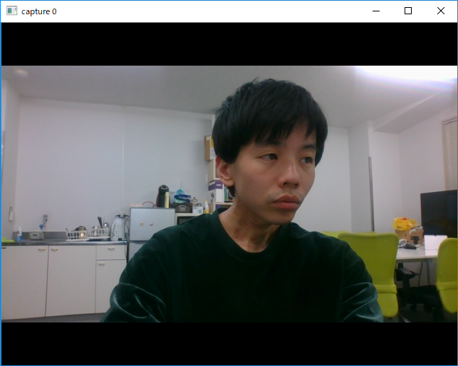
python\camshift.py
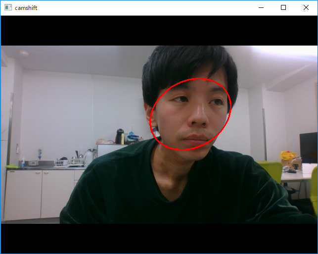
(py36) D:\python-opencv-sample>python camshift.py

Camshift tracker
================

This is a demo that shows mean-shift based tracking
You select a color objects such as your face and it tracks it.
This reads from video camera (0 by default, or the camera number the user enters)

http://www.robinhewitt.com/research/track/camshift.html

Usage:
------
    camshift.py [<video source>]

    To initialize tracking, select the object with mouse

Keys:
-----
    ESC   - exit
    b     - toggle back-projected probability visualization
python\coherence.py
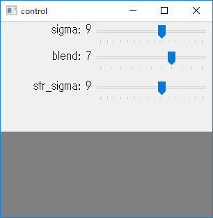
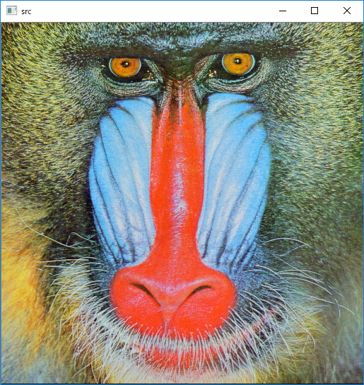
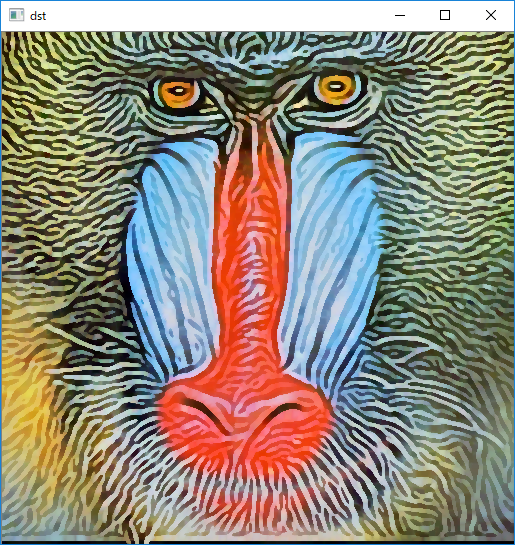
(py36) D:\python-opencv-sample>python coherence.py

Coherence-enhancing filtering example
=====================================

inspired by
  Joachim Weickert "Coherence-Enhancing Shock Filters"
  http://www.mia.uni-saarland.de/Publications/weickert-dagm03.pdf

Press SPACE to update the image

sigma: 19  str_sigma: 19  blend_coef: 0.700000
0
1
2
3
done
Done
python\color_histogram.py
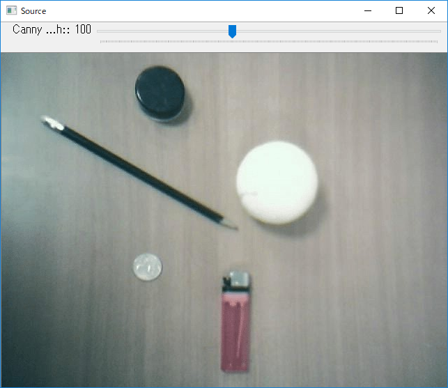
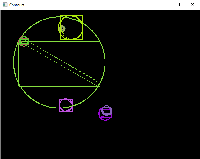
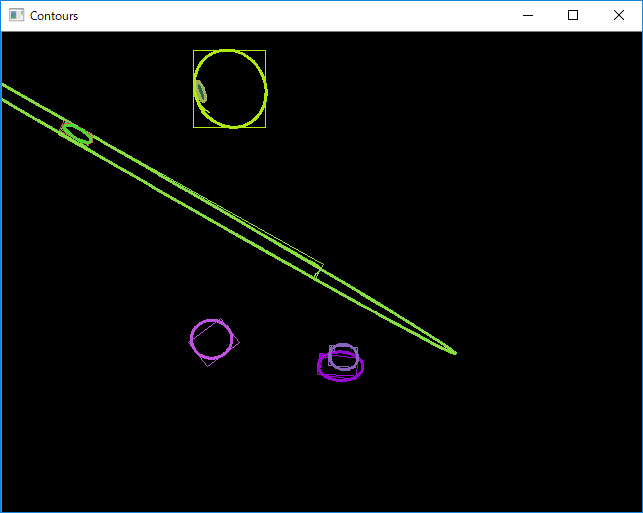
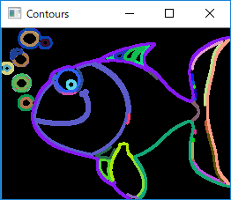
python\contours.py
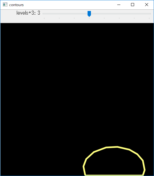
(py36) D:\python-opencv-sample>python contours.py
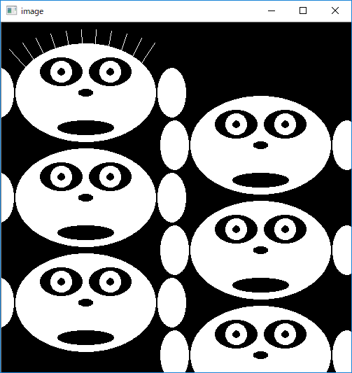
This program illustrates the use of findContours and drawContours.
The original image is put up along with the image of drawn contours.
Usage:
contours.py
A trackbar is put up which controls the contour level from -3 to 3
Done
python\deconvolution.py
python\demo.py
python\dft.py
python\digits.py
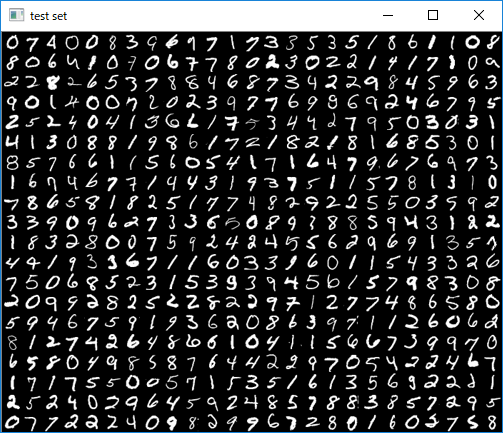
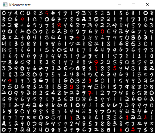
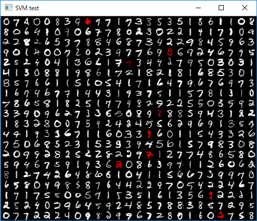
(py36) D:\python-opencv-sample>python digits.py

SVM and KNearest digit recognition.

Sample loads a dataset of handwritten digits from 'digits.png'.
Then it trains a SVM and KNearest classifiers on it and evaluates
their accuracy.

Following preprocessing is applied to the dataset:
 - Moment-based image deskew (see deskew())
 - Digit images are split into 4 10x10 cells and 16-bin
   histogram of oriented gradients is computed for each
   cell
 - Transform histograms to space with Hellinger metric (see [1] (RootSIFT))


[1] R. Arandjelovic, A. Zisserman
    "Three things everyone should know to improve object retrieval"
    http://www.robots.ox.ac.uk/~vgg/publications/2012/Arandjelovic12/arandjelovic12.pdf

Usage:
   digits.py

loading "./data/digits.png" ...
preprocessing...
training KNearest...
error: 3.40 %
confusion matrix:
[[45  0  0  0  0  0  0  0  0  0]
 [ 0 57  0  0  0  0  0  0  0  0]
 [ 0  0 59  1  0  0  0  0  1  0]
 [ 0  0  0 43  0  0  0  1  0  0]
 [ 0  0  0  0 38  0  2  0  0  0]
 [ 0  0  0  2  0 48  0  0  1  0]
 [ 0  1  0  0  0  0 51  0  0  0]
 [ 0  0  1  0  0  0  0 54  0  0]
 [ 0  0  0  0  0  1  0  0 46  0]
 [ 1  1  0  1  1  0  0  0  2 42]]

training SVM...
error: 1.80 %
confusion matrix:
[[45  0  0  0  0  0  0  0  0  0]
 [ 0 57  0  0  0  0  0  0  0  0]
 [ 0  0 59  2  0  0  0  0  0  0]
 [ 0  0  0 43  0  0  0  1  0  0]
 [ 0  0  0  0 40  0  0  0  0  0]
 [ 0  0  0  1  0 50  0  0  0  0]
 [ 0  0  0  0  1  0 51  0  0  0]
 [ 0  0  1  0  0  0  0 54  0  0]
 [ 0  0  0  0  0  0  0  0 47  0]
 [ 0  1  0  1  0  0  0  0  1 45]]

saving SVM as "digits_svm.dat"...
python\digits_adjust.py
(py36) D:\python-opencv-sample>python digits_adjust.py

Digit recognition adjustment.
Grid search is used to find the best parameters for SVM and KNearest classifiers.
SVM adjustment follows the guidelines given in
http://www.csie.ntu.edu.tw/~cjlin/papers/guide/guide.pdf

Usage:
  digits_adjust.py [--model {svm|knearest}]

  --model {svm|knearest}   - select the classifier (SVM is the default)


loading "./data/digits.png" ...
adjusting SVM (may take a long time) ...
.........1 / 225 (best error: 4.16 %, last: 4.16 %)
........
..225 / 225 (best error: 2.82 %, last: 5.02 %)
[[0.31380015 0.12519969 0.07319965 0.06260057 0.05680052 0.0498006
  0.04480064 0.0416002  0.03759968 0.03559996 0.03320008 0.03020008
  0.02840032 0.03       0.05140148]
 [0.13480077 0.07379965 0.06360049 0.0576006  0.0498006  0.04520044
  0.04260036 0.03800008 0.03559996 0.03420012 0.03360036 0.03020044
  0.02820036 0.02860016 0.0502016 ]
 [0.07439989 0.06440069 0.05780068 0.0504006  0.04580056 0.04320024
  0.03940004 0.03740008 0.0354     0.03500068 0.03260092 0.03000048
  0.02820024 0.02860016 0.0502016 ]
 [0.06480049 0.05860064 0.05080064 0.04600052 0.04300016 0.03959988
  0.03720024 0.0362002  0.03620068 0.03400112 0.03320044 0.03020056
  0.02820024 0.02860016 0.0502016 ]
 [0.05920052 0.05160024 0.04600052 0.04360028 0.03960012 0.03700016
  0.03660024 0.03720084 0.037001   0.03540072 0.03220052 0.03000048
  0.02820024 0.02860016 0.0502016 ]
 [0.05180032 0.04580044 0.04380024 0.04100032 0.03700016 0.0370004
  0.03820076 0.03780072 0.03620116 0.03580076 0.03260044 0.03000048
  0.02820024 0.02860016 0.0502016 ]
 [0.04700032 0.0436004  0.04100032 0.03700016 0.03840036 0.03800044
  0.0396006  0.03760052 0.036401   0.03560044 0.03300036 0.03000048
  0.02820024 0.02860016 0.0502016 ]
 [0.0434002  0.04220032 0.0374002  0.03820028 0.0376004  0.04060052
  0.03900084 0.03760052 0.036401   0.03620044 0.03300036 0.03000048
  0.02820024 0.02860016 0.0502016 ]
 [0.04240016 0.03780024 0.0382004  0.03820028 0.04040044 0.04000064
  0.03960072 0.03660072 0.03680092 0.03620044 0.03300036 0.03000048
  0.02820024 0.02860016 0.0502016 ]
 [0.03880028 0.03800032 0.03800032 0.04040032 0.04060076 0.04100056
  0.03880076 0.03720084 0.03680092 0.03620044 0.03300036 0.03000048
  0.02820024 0.02860016 0.0502016 ]
 [0.03780012 0.03840036 0.03980032 0.04120076 0.04160044 0.04080072
  0.03940088 0.03740068 0.03680092 0.03620044 0.03300036 0.03000048
  0.02820024 0.02860016 0.0502016 ]
 [0.03900048 0.03940028 0.04180088 0.04140048 0.04100044 0.04080072
  0.04020072 0.03740068 0.03680092 0.03620044 0.03300036 0.03000048
  0.02820024 0.02860016 0.0502016 ]
 [0.03920044 0.04220092 0.04160044 0.04080036 0.04140072 0.04280056
  0.04040068 0.03740068 0.03680092 0.03620044 0.03300036 0.03000048
  0.02820024 0.02860016 0.0502016 ]
 [0.04200084 0.0420006  0.0412004  0.04300076 0.04400068 0.04340068
  0.04040068 0.03740068 0.03680092 0.03620044 0.03300036 0.03000048
  0.02820024 0.02860016 0.0502016 ]
 [0.04220092 0.04140036 0.04300076 0.04360064 0.04460056 0.04340068
  0.04040068 0.03740068 0.03680092 0.03620044 0.03300036 0.03000048
  0.02820024 0.02860016 0.0502016 ]]
writing score table to "svm_scores.npz"
best params: {'C': 2.6918003852647123, 'gamma': 5.3836007705294255}
best error: 2.82 %
work time: 60.748085 s
python\digits_video.py
(py36) D:\python-opencv-sample>python digits_video.py
None
Done
[ WARN:0] terminating async callback
python\distrans.py
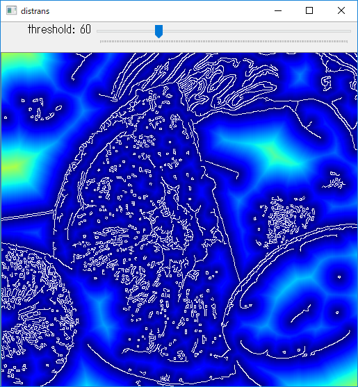
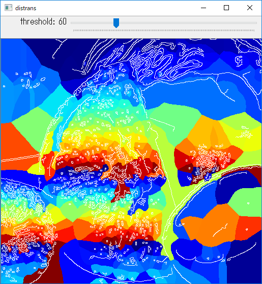
(py36) D:\python-opencv-sample>python distrans.py

Distance transform sample.

Usage:
  distrans.py [<image>]

Keys:
  ESC   - exit
  v     - toggle voronoi mode

showing voronoi
Done
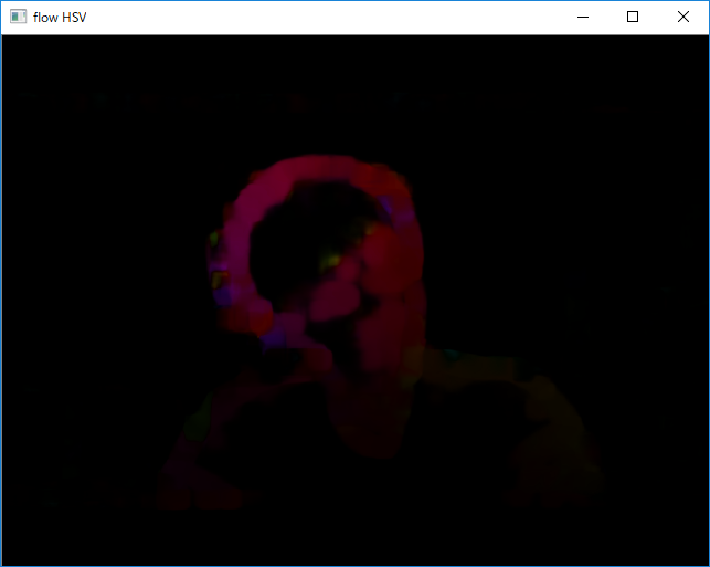
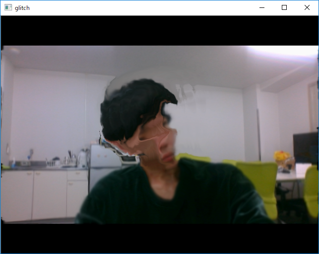
python\dis_opt_flow.py
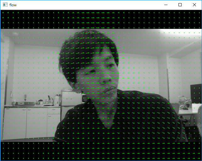
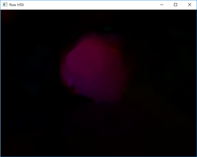
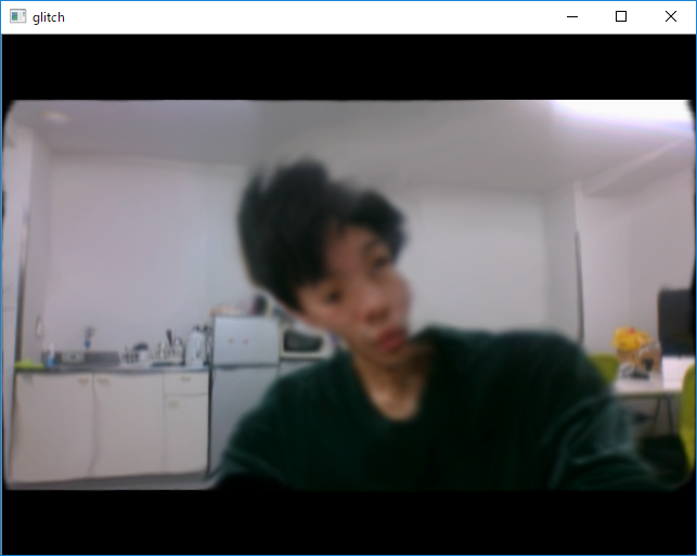
(py36) D:\python-opencv-sample>python dis_opt_flow.py

example to show optical flow estimation using DISOpticalFlow

USAGE: dis_opt_flow.py [<video_source>]

Keys:
 1  - toggle HSV flow visualization
 2  - toggle glitch
 3  - toggle spatial propagation of flow vectors
 4  - toggle temporal propagation of flow vectors
ESC - exit


example to show optical flow estimation using DISOpticalFlow

USAGE: dis_opt_flow.py [<video_source>]

Keys:
 1  - toggle HSV flow visualization
 2  - toggle glitch
 3  - toggle spatial propagation of flow vectors
 4  - toggle temporal propagation of flow vectors
ESC - exit

HSV flow visualization is on
glitch is off
glitch is on
temporal propagation is off
temporal propagation is on
Done
[ WARN:0] terminating async callback
python\edge.py
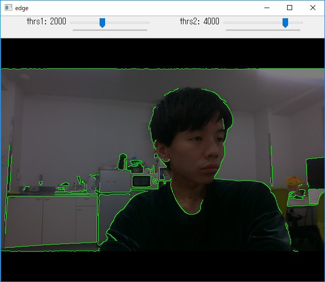
(py36) D:\python-opencv-sample>python edge.py

This sample demonstrates Canny edge detection.

Usage:
  edge.py [<video source>]

  Trackbars control edge thresholds.


Done
[ WARN:0] terminating async callback
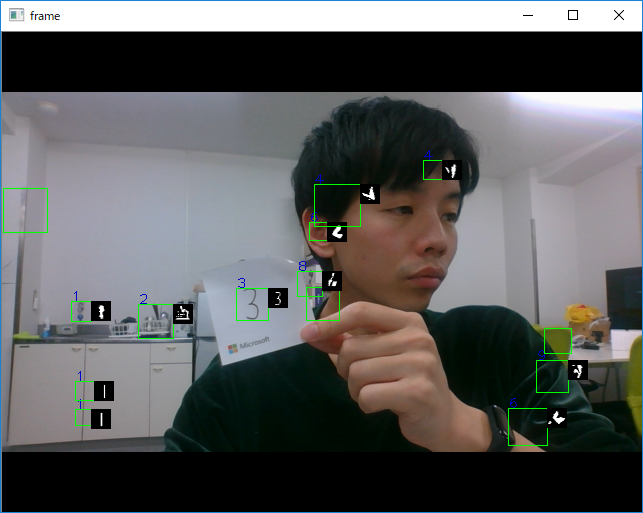
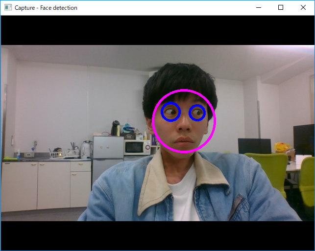
python\facedetect.py
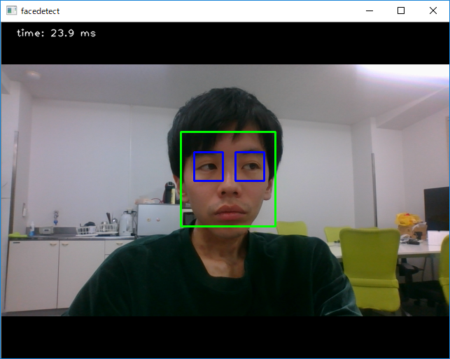
(py36) D:\python-opencv-sample>python facedetect.py

face detection using haar cascades

USAGE:
    facedetect.py [--cascade <cascade_fn>] [--nested-cascade <cascade_fn>] [<video_source>]

Done
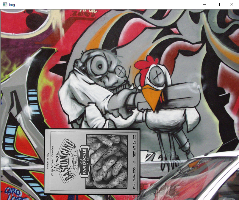
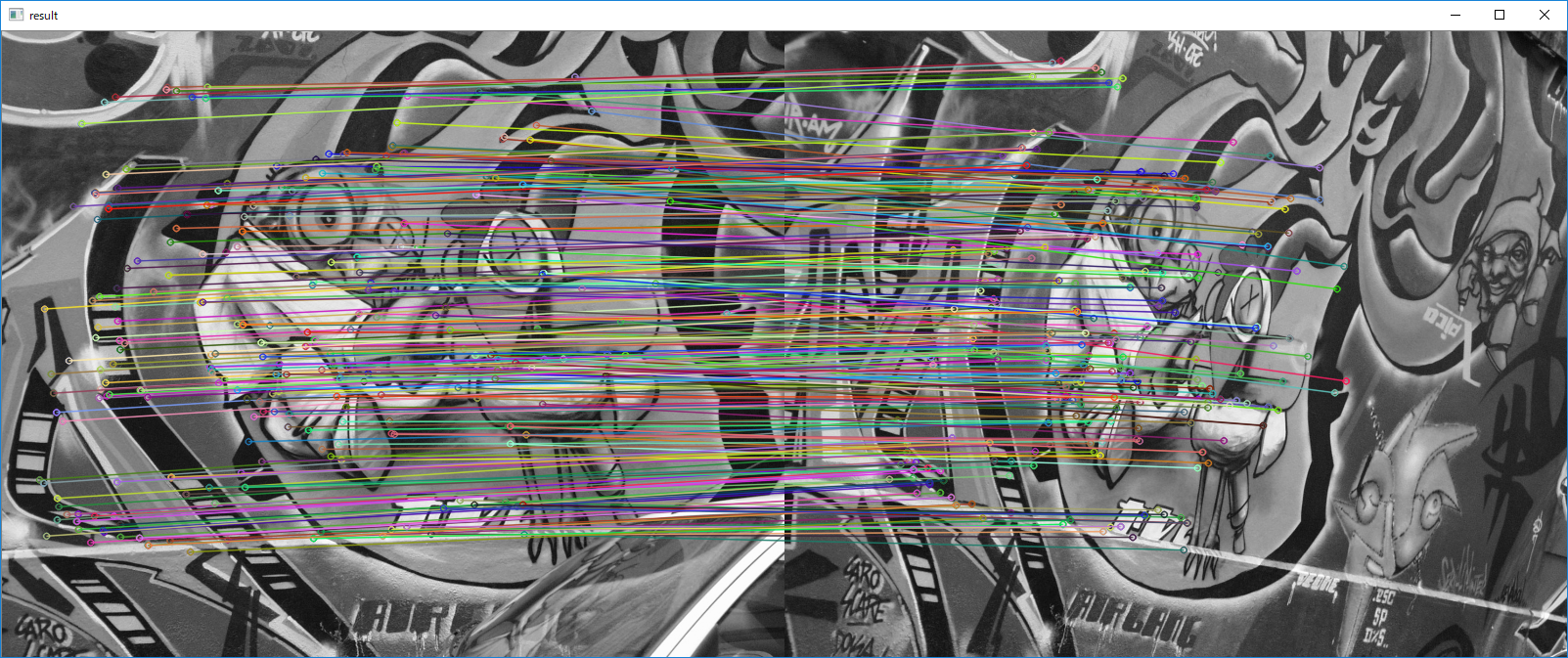
python\feature_homography.py
(py36) D:\python-opencv-sample>python feature_homography.py

Feature homography
==================

Example of using features2d framework for interactive video homography matching.
ORB features and FLANN matcher are used. The actual tracking is implemented by
PlaneTracker class in plane_tracker.py

Inspired by http://www.youtube.com/watch?v=-ZNYoL8rzPY

video: http://www.youtube.com/watch?v=FirtmYcC0Vc

Usage
-----
feature_homography.py [<video source>]

Keys:
   SPACE  -  pause video

Select a textured planar object to track by drawing a box with a mouse.
python\find_obj.py
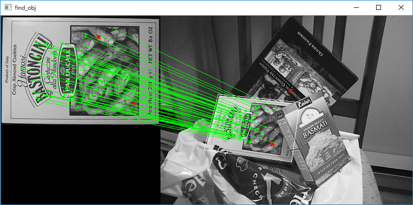
(py36) D:\python-opencv-sample>python find_obj.py

Feature-based image matching sample.

Note, that you will need the https://github.com/opencv/opencv_contrib repo for SIFT and SURF

USAGE
  find_obj.py [--feature=<sift|surf|orb|akaze|brisk>[-flann]] [ <image1> <image2> ]

  --feature  - Feature to use. Can be sift, surf, orb or brisk. Append '-flann'
               to feature name to use Flann-based matcher instead bruteforce.

  Press left mouse button on a feature point to see its matching point.

using brisk
img1 - 1662 features, img2 - 2786 features
matching...
50 / 52  inliers/matched
Done
python\fitline.py
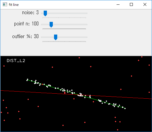
(py36) D:\python-opencv-sample>python fitline.py

Robust line fitting.
==================

Example of using cv.fitLine function for fitting line
to points in presence of outliers.

Usage
-----
fitline.py

Switch through different M-estimator functions and see,
how well the robust functions fit the line even
in case of ~50% of outliers.

Keys
----
SPACE - generate random points
f     - change distance function
ESC   - exit

Done
python\floodfill.py
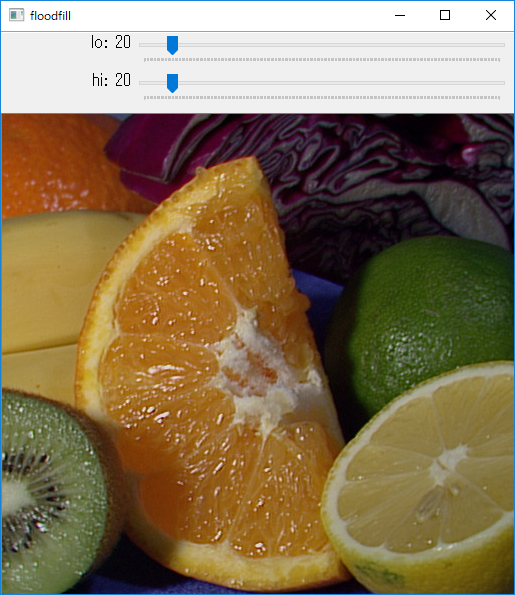
(py36) D:\python-opencv-sample>python floodfill.py

Floodfill sample.

Usage:
  floodfill.py [<image>]

  Click on the image to set seed point

Keys:
  f     - toggle floating range
  c     - toggle 4/8 connectivity
  ESC   - exit

Done
python\gabor_threads.py

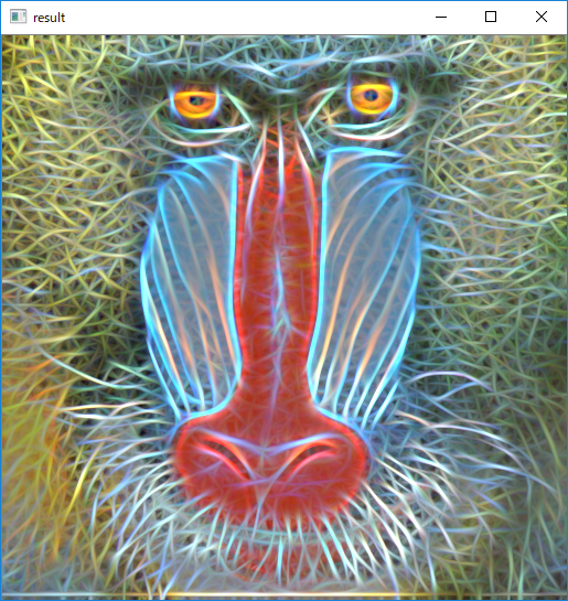
(py36) D:\python-opencv-sample>python gabor_threads.py

gabor_threads.py
=========

Sample demonstrates:
- use of multiple Gabor filter convolutions to get Fractalius-like image effect (http://www.redfieldplugins.com/filterFractalius.htm)
- use of python threading to accelerate the computation

Usage
-----
gabor_threads.py [image filename]


running single-threaded ...
354.46 ms
running multi-threaded ...
61.23 ms
res1 == res2:  True
Done
python\gaussian_mix.py
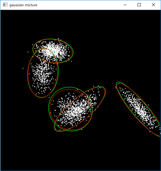
(py36) D:\python-opencv-sample>python gaussian_mix.py
None
press any key to update distributions, ESC - exit

sampling distributions...
EM (opencv) ...
ready!

Done
python\grabcut.py
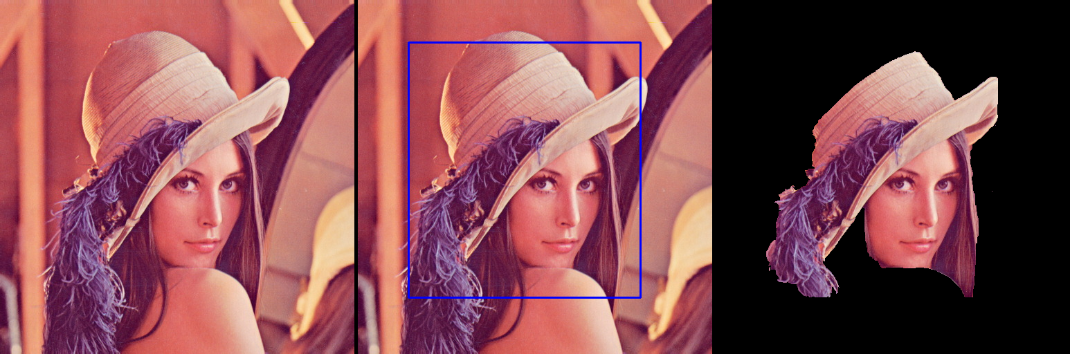
(py36) D:\python-opencv-sample>python grabcut.py

===============================================================================
Interactive Image Segmentation using GrabCut algorithm.

This sample shows interactive image segmentation using grabcut algorithm.

USAGE:
    python grabcut.py <filename>

README FIRST:
    Two windows will show up, one for input and one for output.

    At first, in input window, draw a rectangle around the object using
mouse right button. Then press 'n' to segment the object (once or a few times)
For any finer touch-ups, you can press any of the keys below and draw lines on
the areas you want. Then again press 'n' for updating the output.

Key '0' - To select areas of sure background
Key '1' - To select areas of sure foreground
Key '2' - To select areas of probable background
Key '3' - To select areas of probable foreground

Key 'n' - To update the segmentation
Key 'r' - To reset the setup
Key 's' - To save the results
===============================================================================

No input image given, so loading default image, lena.jpg

Correct Usage: python grabcut.py <filename>

 Instructions:

 Draw a rectangle around the object using right mouse button

 Now press the key 'n' a few times until no further change

 For finer touchups, mark foreground and background after pressing keys 0-3
                and again press 'n'

 Result saved as image

Done
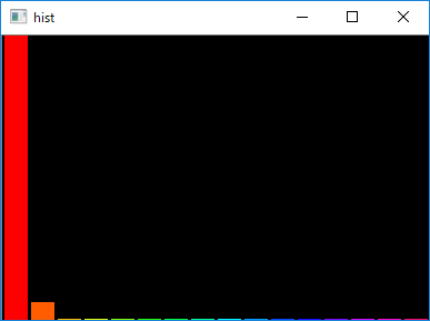
python\hist.py
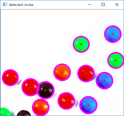
python\houghcircles.py
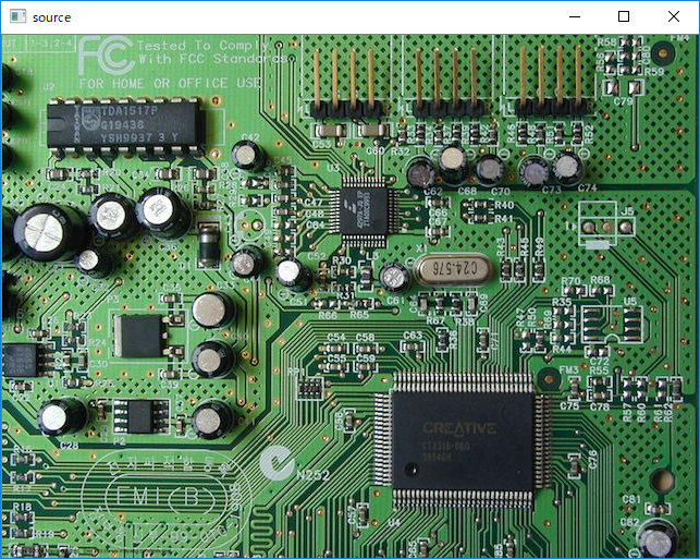
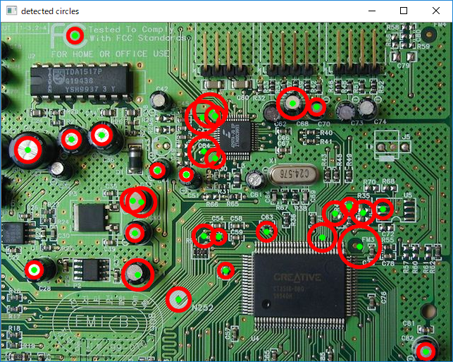
(py36) D:\python-opencv-sample>python houghcircles.py

This example illustrates how to use cv.HoughCircles() function.

Usage:
    houghcircles.py [<image_name>]
    image argument defaults to board.jpg

Done
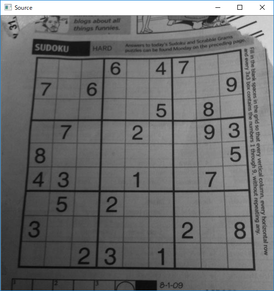
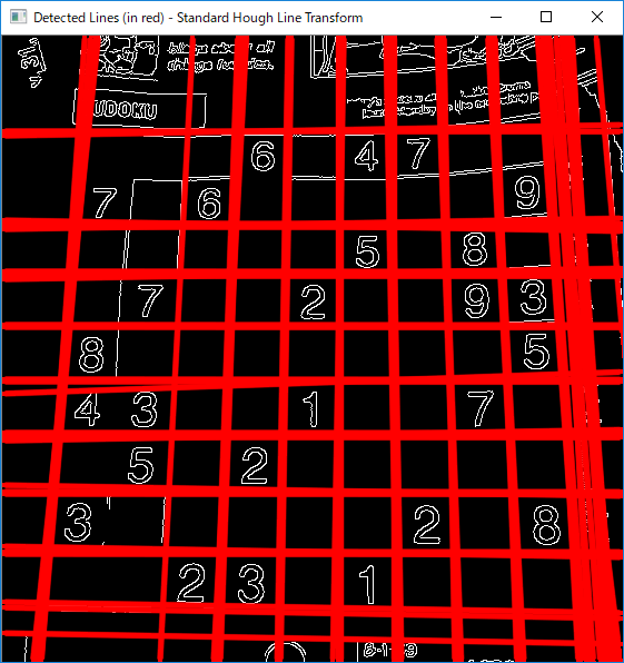
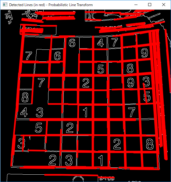
python\houghlines.py
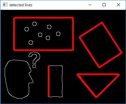
(py36) D:\python-opencv-sample>python houghlines.py

This example illustrates how to use Hough Transform to find lines

Usage:
    houghlines.py [<image_name>]
    image argument defaults to pic1.png

Done
python\inpaint.py
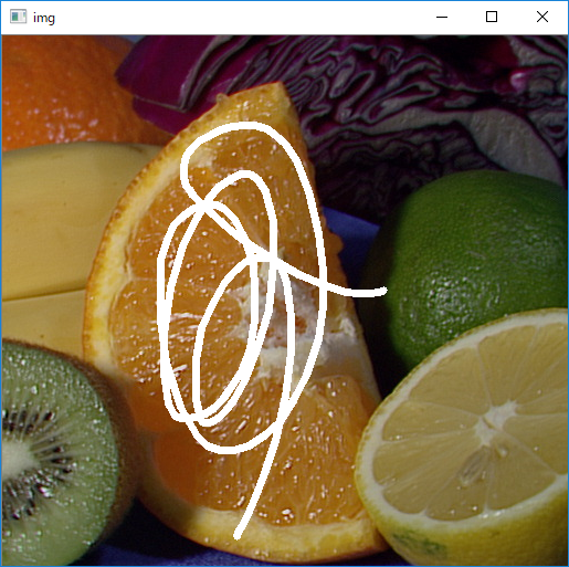
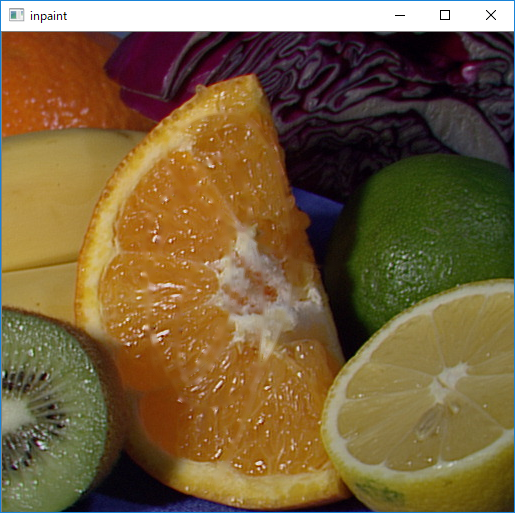
(py36) D:\python-opencv-sample>python inpaint.py

Inpainting sample.

Inpainting repairs damage to images by floodfilling
the damage with surrounding image areas.

Usage:
  inpaint.py [<image>]

Keys:
  SPACE - inpaint
  r     - reset the inpainting mask
  ESC   - exit

Done
python\kalman.py
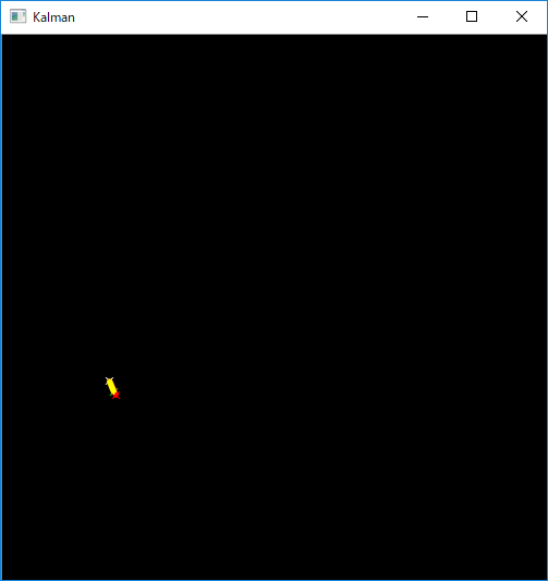
(py36) D:\python-opencv-sample>python kalman.py

   Tracking of rotating point.
   Rotation speed is constant.
   Both state and measurements vectors are 1D (a point angle),
   Measurement is the real point angle + gaussian noise.
   The real and the estimated points are connected with yellow line segment,
   the real and the measured points are connected with red line segment.
   (if Kalman filter works correctly,
    the yellow segment should be shorter than the red one).
   Pressing any key (except ESC) will reset the tracking with a different speed.
   Pressing ESC will stop the program.

Done
python\kmeans.py
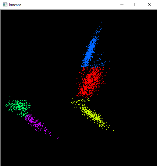
(py36) D:\python-opencv-sample>python kmeans.py

K-means clusterization sample.
Usage:
   kmeans.py

Keyboard shortcuts:
   ESC   - exit
   space - generate new distribution

sampling distributions...
Done
python\lappyr.py
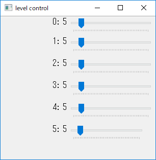
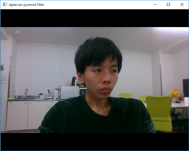
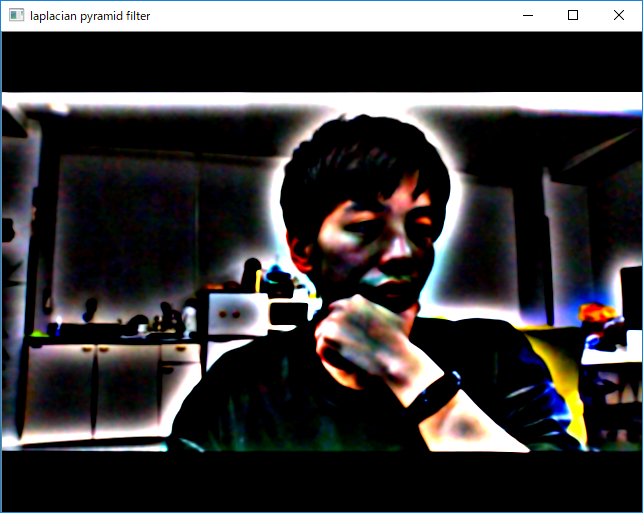
(py36) D:\python-opencv-sample>python lappyr.py
 An example of Laplacian Pyramid construction and merging.

Level : Intermediate

Usage : python lappyr.py [<video source>]

References:
  http://citeseerx.ist.psu.edu/viewdoc/summary?doi=10.1.1.54.299

Alexander Mordvintsev 6/10/12

Done
[ WARN:0] terminating async callback
python\letter_recog.py
(py36) D:\python-opencv-sample>python letter_recog.py

The sample demonstrates how to train Random Trees classifier
(or Boosting classifier, or MLP, or Knearest, or Support Vector Machines) using the provided dataset.

We use the sample database letter-recognition.data
from UCI Repository, here is the link:

Newman, D.J. & Hettich, S. & Blake, C.L. & Merz, C.J. (1998).
UCI Repository of machine learning databases
[http://www.ics.uci.edu/~mlearn/MLRepository.html].
Irvine, CA: University of California, Department of Information and Computer Science.

The dataset consists of 20000 feature vectors along with the
responses - capital latin letters A..Z.
The first 10000 samples are used for training
and the remaining 10000 - to test the classifier.
======================================================
USAGE:
  letter_recog.py [--model <model>]
                  [--data <data fn>]
                  [--load <model fn>] [--save <model fn>]

  Models: RTrees, KNearest, Boost, SVM, MLP

loading data ./data/letter-recognition.data ...
training SVM ...
testing...
train rate: 99.780000  test rate: 95.690000
Done
python\lk_homography.py

(py36) D:\python-opencv-sample>python lk_homography.py

Lucas-Kanade homography tracker
===============================

Lucas-Kanade sparse optical flow demo. Uses goodFeaturesToTrack
for track initialization and back-tracking for match verification
between frames. Finds homography between reference and current views.

Usage
-----
lk_homography.py [<video_source>]


Keys
----
ESC   - exit
SPACE - start tracking
r     - toggle RANSAC

[ WARN:0] terminating async callback
Done
python\lk_track.py
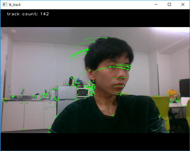
(py36) D:\python-opencv-sample>python lk_track.py

Lucas-Kanade tracker
====================

Lucas-Kanade sparse optical flow demo. Uses goodFeaturesToTrack
for track initialization and back-tracking for match verification
between frames.

Usage
-----
lk_track.py [<video_source>]


Keys
----
ESC - exit

[ WARN:0] terminating async callback
Done
python\logpolar.py

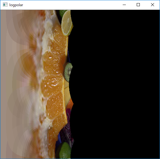
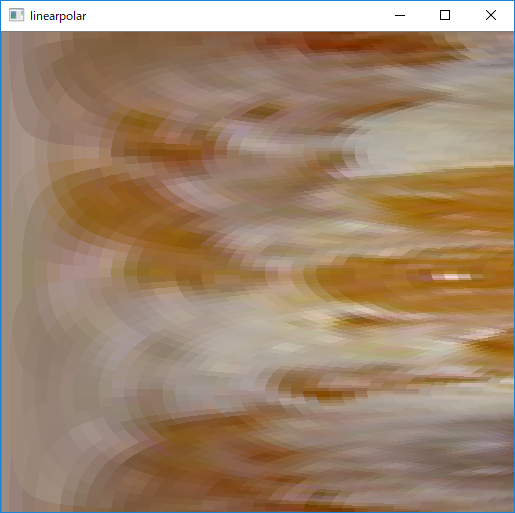
(py36) D:\python-opencv-sample>python logpolar.py

plots image as logPolar and linearPolar

Usage:
    logpolar.py

Keys:
    ESC    - exit

Done
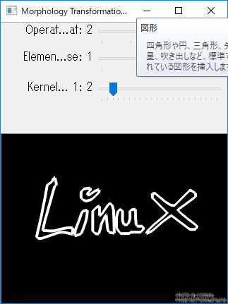
python\morphology.py

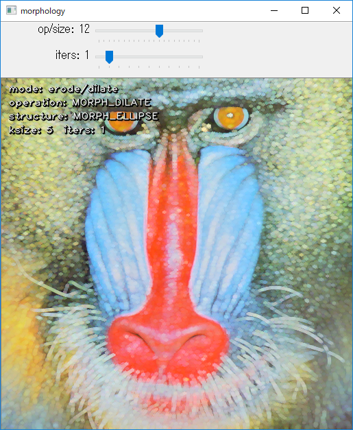
(py36) D:\python-opencv-sample>python morphology.py

Morphology operations.

Usage:
  morphology.py [<image>]

Keys:
  1   - change operation
  2   - change structure element shape
  ESC - exit

Done
python\mosse.py
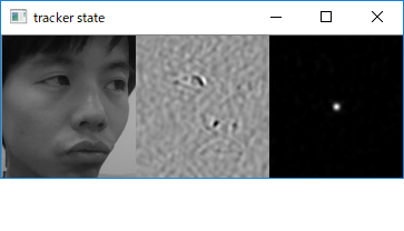
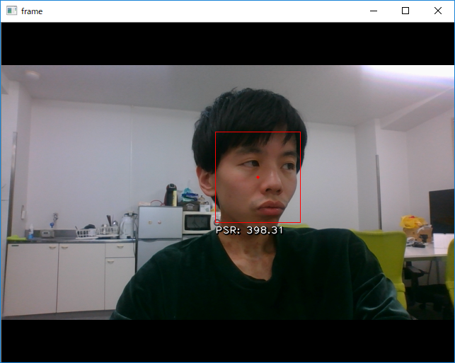
(py36) D:\python-opencv-sample>python mosse.py

MOSSE tracking sample

This sample implements correlation-based tracking approach, described in [1].

Usage:
  mosse.py [--pause] [<video source>]

  --pause  -  Start with playback paused at the first video frame.
              Useful for tracking target selection.

  Draw rectangles around objects with a mouse to track them.

Keys:
  SPACE    - pause video
  c        - clear targets

[1] David S. Bolme et al. "Visual Object Tracking using Adaptive Correlation Filters"
    http://www.cs.colostate.edu/~draper/papers/bolme_cvpr10.pdf
python\mouse_and_match.py
python\mser.py
(py36) D:\python-opencv-sample>python mser.py

MSER detector demo
==================

Usage:
------
    mser.py [<video source>]

Keys:
-----
    ESC   - exit


Done
[ WARN:0] terminating async callback
python\opencv_version.py
(py36) D:\python-opencv-sample>python opencv_version.py

prints OpenCV version

Usage:
    opencv_version.py [<params>]
    params:
        --build: print complete build info
        --help:  print this help

Welcome to OpenCV
Done
(py36) D:\python-opencv-sample>python opencv_version.py --build

prints OpenCV version

Usage:
    opencv_version.py [<params>]
    params:
        --build: print complete build info
        --help:  print this help


General configuration for OpenCV 4.0.0 =====================================
  Version control:               4.0.0

  Platform:
    Timestamp:                   2019-01-09T18:51:15Z
    Host:                        Windows 6.3.9600 AMD64
    CMake:                       3.12.2
    CMake generator:             Visual Studio 14 2015 Win64
    CMake build tool:            C:/Program Files (x86)/MSBuild/14.0/bin/MSBuild.exe
    MSVC:                        1900

  CPU/HW features:
    Baseline:                    SSE SSE2 SSE3
      requested:                 SSE3
    Dispatched code generation:  SSE4_1 SSE4_2 FP16 AVX AVX2
      requested:                 SSE4_1 SSE4_2 AVX FP16 AVX2 AVX512_SKX
      SSE4_1 (5 files):          + SSSE3 SSE4_1
      SSE4_2 (1 files):          + SSSE3 SSE4_1 POPCNT SSE4_2
      FP16 (0 files):            + SSSE3 SSE4_1 POPCNT SSE4_2 FP16 AVX
      AVX (4 files):             + SSSE3 SSE4_1 POPCNT SSE4_2 AVX
      AVX2 (11 files):           + SSSE3 SSE4_1 POPCNT SSE4_2 FP16 FMA3 AVX AVX2

  C/C++:
    Built as dynamic libs?:      NO
    C++ Compiler:                C:/Program Files (x86)/Microsoft Visual Studio 14.0/VC/bin/x86_amd64/cl.exe  (ver 19.0.24241.7)
    C++ flags (Release):         /DWIN32 /D_WINDOWS /W4 /GR  /D _CRT_SECURE_NO_DEPRECATE /D _CRT_NONSTDC_NO_DEPRECATE /D _SCL_SECURE_NO_WARNINGS /Gy /bigobj /Oi      /EHa /wd4127 /wd4251 /wd4324 /wd4275 /wd4512 /wd4589 /MP2   /MT /O2 /Ob2 /DNDEBUG
    C++ flags (Debug):           /DWIN32 /D_WINDOWS /W4 /GR  /D _CRT_SECURE_NO_DEPRECATE /D _CRT_NONSTDC_NO_DEPRECATE /D _SCL_SECURE_NO_WARNINGS /Gy /bigobj /Oi      /EHa /wd4127 /wd4251 /wd4324 /wd4275 /wd4512 /wd4589 /MP2   /MTd /Zi /Ob0 /Od /RTC1
    C Compiler:                  C:/Program Files (x86)/Microsoft Visual Studio 14.0/VC/bin/x86_amd64/cl.exe
    C flags (Release):           /DWIN32 /D_WINDOWS /W3  /D _CRT_SECURE_NO_DEPRECATE /D _CRT_NONSTDC_NO_DEPRECATE /D _SCL_SECURE_NO_WARNINGS /Gy /bigobj /Oi        /MP2    /MT /O2 /Ob2 /DNDEBUG
    C flags (Debug):             /DWIN32 /D_WINDOWS /W3  /D _CRT_SECURE_NO_DEPRECATE /D _CRT_NONSTDC_NO_DEPRECATE /D _SCL_SECURE_NO_WARNINGS /Gy /bigobj /Oi        /MP2  /MTd /Zi /Ob0 /Od /RTC1
    Linker flags (Release):      /machine:x64  /NODEFAULTLIB:atlthunk.lib /INCREMENTAL:NO  /NODEFAULTLIB:libcmtd.lib /NODEFAULTLIB:libcpmtd.lib /NODEFAULTLIB:msvcrtd.lib
    Linker flags (Debug):        /machine:x64  /NODEFAULTLIB:atlthunk.lib /debug /INCREMENTAL  /NODEFAULTLIB:libcmt.lib /NODEFAULTLIB:libcpmt.lib /NODEFAULTLIB:msvcrt.lib
    ccache:                      NO
    Precompiled headers:         YES
    Extra dependencies:          ade comctl32 gdi32 ole32 setupapi ws2_32
    3rdparty dependencies:       ittnotify libprotobuf zlib libjpeg-turbo libwebp libpng libtiff libjasper IlmImf quirc ippiw ippicv

  OpenCV modules:
    To be built:                 calib3d core dnn features2d flann gapi highgui imgcodecs imgproc java_bindings_generator ml objdetect photo python3 python_bindings_generator stitching video videoio
    Disabled:                    world
    Disabled by dependency:      -
    Unavailable:                 java js python2 ts
    Applications:                -
    Documentation:               NO
    Non-free algorithms:         NO

  Windows RT support:            NO

  GUI:
    Win32 UI:                    YES
    VTK support:                 NO

  Media I/O:
    ZLib:                        build (ver 1.2.11)
    JPEG:                        build-libjpeg-turbo (ver 1.5.3-62)
    WEBP:                        build (ver encoder: 0x020e)
    PNG:                         build (ver 1.6.35)
    TIFF:                        build (ver 42 - 4.0.9)
    JPEG 2000:                   build (ver 1.900.1)
    OpenEXR:                     build (ver 1.7.1)
    HDR:                         YES
    SUNRASTER:                   YES
    PXM:                         YES
    PFM:                         YES

  Video I/O:
    DC1394:                      NO
    FFMPEG:                      YES (prebuilt binaries)
      avcodec:                   YES (ver 58.35.100)
      avformat:                  YES (ver 58.20.100)
      avutil:                    YES (ver 56.22.100)
      swscale:                   YES (ver 5.3.100)
      avresample:                YES (ver 4.0.0)
    GStreamer:                   NO
    DirectShow:                  YES
    Media Foundation:            YES

  Parallel framework:            Concurrency

  Trace:                         YES (with Intel ITT)

  Other third-party libraries:
    Intel IPP:                   2019.0.0 Gold [2019.0.0]
           at:                   C:/projects/opencv-python/_skbuild/win-amd64-3.6/cmake-build/3rdparty/ippicv/ippicv_win/icv
    Intel IPP IW:                sources (2019.0.0)
              at:                C:/projects/opencv-python/_skbuild/win-amd64-3.6/cmake-build/3rdparty/ippicv/ippicv_win/iw
    Lapack:                      NO
    Eigen:                       NO
    Custom HAL:                  NO
    Protobuf:                    build (3.5.1)

  OpenCL:                        YES (no extra features)
    Include path:                C:/projects/opencv-python/opencv/3rdparty/include/opencl/1.2
    Link libraries:              Dynamic load

  Python 3:
    Interpreter:                 C:/Python36-x64/python.exe (ver 3.6.6)
    Libraries:                   C:/Python36-x64/libs/python36.lib (ver 3.6.6)
    numpy:                       C:/Python36-x64/lib/site-packages/numpy/core/include (ver 1.11.3)
    packages path:               C:/Python36-x64/Lib/site-packages

  Python (for build):            C:/Python27-x64/python.exe

  Java:
    ant:                         NO
    JNI:                         C:/Program Files/Java/jdk1.8.0/include C:/Program Files/Java/jdk1.8.0/include/win32 C:/Program Files/Java/jdk1.8.0/include
    Java wrappers:               NO
    Java tests:                  NO

  Install to:                    C:/projects/opencv-python/_skbuild/win-amd64-3.6/cmake-install
-----------------------------------------------------------------


Done
python\opt_flow.py
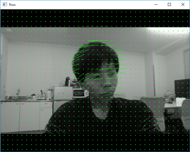
(py36) D:\python-opencv-sample>python opt_flow.py

example to show optical flow

USAGE: opt_flow.py [<video_source>]

Keys:
 1 - toggle HSV flow visualization
 2 - toggle glitch

Keys:
    ESC    - exit

HSV flow visualization is on
opt_flow.py:42: RuntimeWarning: invalid value encountered in sqrt
  v = np.sqrt(fx*fx+fy*fy)
glitch is on
glitch is off
glitch is on
Done
[ WARN:0] terminating async callback
python\peopledetect.py
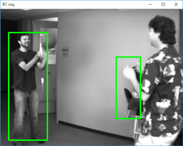
(py36) D:\python-opencv-sample>python peopledetect.py

example to detect upright people in images using HOG features

Usage:
    peopledetect.py <image_names>

Press any key to continue, ESC to stop.

./data/basketball2.png  -
2 (2) found
Done
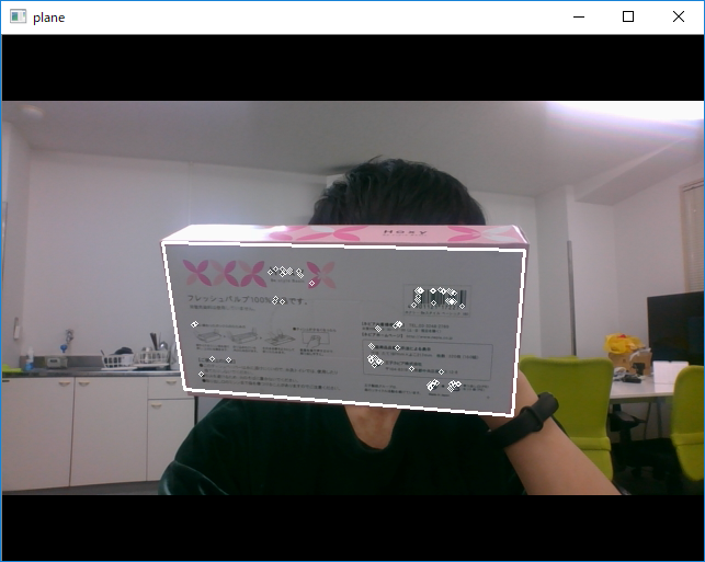
python\plane_ar.py
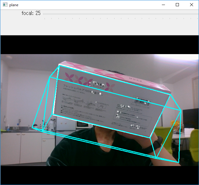
(py36) D:\python-opencv-sample>python plane_ar.py

Planar augmented reality
==================

This sample shows an example of augmented reality overlay over a planar object
tracked by PlaneTracker from plane_tracker.py. solvePnP function is used to
estimate the tracked object location in 3d space.

video: http://www.youtube.com/watch?v=pzVbhxx6aog

Usage
-----
plane_ar.py [<video source>]

Keys:
   SPACE  -  pause video
   c      -  clear targets

Select a textured planar object to track by drawing a box with a mouse.
Use 'focal' slider to adjust to camera focal length for proper video augmentation.
python\plane_tracker.py
(py36) D:\python-opencv-sample>python plane_tracker.py

Multitarget planar tracking
==================

Example of using features2d framework for interactive video homography matching.
ORB features and FLANN matcher are used. This sample provides PlaneTracker class
and an example of its usage.

video: http://www.youtube.com/watch?v=pzVbhxx6aog

Usage
-----
plane_tracker.py [<video source>]

Keys:
   SPACE  -  pause video
   c      -  clear targets

Select a textured planar object to track by drawing a box with a mouse.
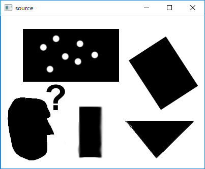
python\squares.py
(py36) D:\python-opencv-sample>python squares.py

Simple "Square Detector" program.

Loads several images sequentially and tries to find squares in each image.

Done
python\stereo_match.py
python\stitching.py
python\stitching_detailed.py
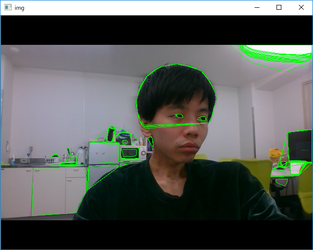
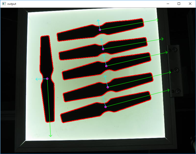
python\texture_flow.py
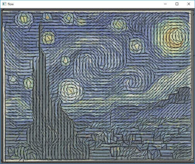
(py36) D:\python-opencv-sample>python texture_flow.py

Texture flow direction estimation.

Sample shows how cv.cornerEigenValsAndVecs function can be used
to estimate image texture flow direction.

Usage:
    texture_flow.py [<image>]

Done
python\tst_scene_render.py
(py36) D:\python-opencv-sample>python tst_scene_render.py
None
Done
python\turing.py
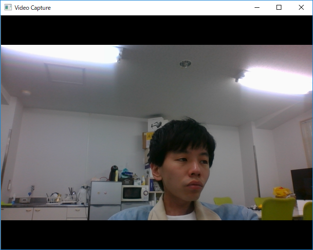
python\video.py
(py36) D:\python-opencv-sample>python video.py

Video capture sample.

Sample shows how VideoCapture class can be used to acquire video
frames from a camera of a movie file. Also the sample provides
an example of procedural video generation by an object, mimicking
the VideoCapture interface (see Chess class).

'create_capture' is a convenience function for capture creation,
falling back to procedural video in case of error.

Usage:
    video.py [--shotdir <shot path>] [source0] [source1] ...'

    sourceN is an
     - integer number for camera capture
     - name of video file
     - synth:<params> for procedural video

Synth examples:
    synth:bg=lena.jpg:noise=0.1
    synth:class=chess:bg=lena.jpg:noise=0.1:size=640x480

Keys:
    ESC    - exit
    SPACE  - save current frame to <shot path> directory


./shot_0_000.bmp saved
[ WARN:0] terminating async callback
python\video_threaded.py
(py36) D:\python-opencv-sample>python video_threaded.py

Multithreaded video processing sample.
Usage:
   video_threaded.py {<video device number>|<video file name>}

   Shows how python threading capabilities can be used
   to organize parallel captured frame processing pipeline
   for smoother playback.

Keyboard shortcuts:

   ESC - exit
   space - switch between multi and single threaded processing

Done
[ WARN:0] terminating async callback
python\video_v4l2.py
(py36) D:\python-opencv-sample>python video_v4l2.py

VideoCapture sample showcasing  some features of the Video4Linux2 backend

Sample shows how VideoCapture class can be used to control parameters
of a webcam such as focus or framerate.
Also the sample provides an example how to access raw images delivered
by the hardware to get a grayscale image in a very efficient fashion.

Keys:
    ESC    - exit
    g      - toggle optimized grayscale conversion
python\watershed.py
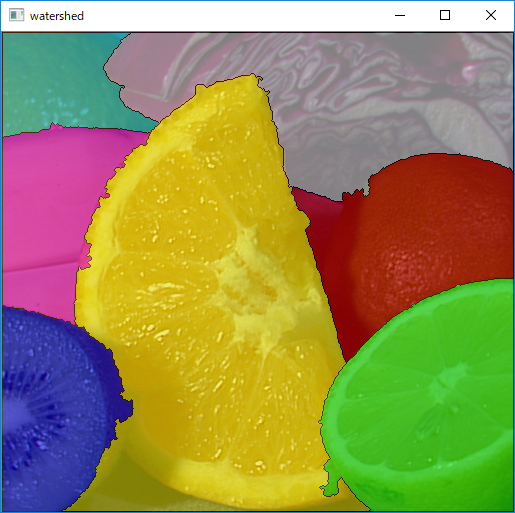
(py36) D:\python-opencv-sample>python watershed.py

Watershed segmentation
=========

This program demonstrates the watershed segmentation algorithm
in OpenCV: watershed().

Usage
-----
watershed.py [image filename]

Keys
----
  1-7   - switch marker color
  SPACE - update segmentation
  r     - reset
  a     - toggle autoupdate
  ESC   - exit


marker:  1
marker:  2
marker:  3
marker:  4
marker:  5
marker:  6
marker:  7
marker:  3
marker:  1
marker:  7
python_coverage.py
(py36) D:\python-opencv-sample>python _coverage.py
 ---  asift.py
 ---  browse.py
 ---  calibrate.py
 ---  camera_calibration_show_extrinsics.py
 ---  camshift.py
 ---  coherence.py
 ---  color_histogram.py
 ---  common.py
 ---  contours.py
 ---  deconvolution.py
 ---  demo.py
 ---  dft.py
 ---  digits.py
 ---  digits_adjust.py
 ---  digits_video.py
 ---  distrans.py
 ---  dis_opt_flow.py
 ---  edge.py
 ---  facedetect.py
 ---  feature_homography.py
 ---  find_obj.py
 ---  fitline.py
 ---  floodfill.py
 ---  gabor_threads.py
 ---  gaussian_mix.py
 ---  grabcut.py
 ---  hist.py
 ---  houghcircles.py
 ---  houghlines.py
 ---  inpaint.py
 ---  kalman.py
 ---  kmeans.py
 ---  lappyr.py
 ---  letter_recog.py
 ---  lk_homography.py
 ---  lk_track.py
 ---  logpolar.py
 ---  morphology.py
 ---  mosse.py
 ---  mouse_and_match.py
 ---  mser.py
 ---  opencv_version.py
 ---  opt_flow.py
 ---  peopledetect.py
 ---  plane_ar.py
 ---  plane_tracker.py
 ---  squares.py
 ---  stereo_match.py
 ---  stitching.py
 ---  stitching_detailed.py
 ---  texture_flow.py
 ---  tst_scene_render.py
 ---  turing.py
 ---  video.py
 ---  video_threaded.py
 ---  video_v4l2.py
 ---  watershed.py
 ---  _coverage.py
 ---  _doc.py

cv api coverage: 125 / 470  (26.6%)
python_doc.py
(py36) D:\python-opencv-sample>python _doc.py
--- undocumented files:
camera_calibration_show_extrinsics.py
digits_video.py
gaussian_mix.py
tst_scene_render.py
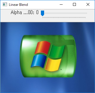
python\tutorial_code\core\AddingImages\adding_images.py

(py36) D:\python-opencv-sample\tutorial_code\core\AddingImages>python adding_images.py
 Simple Linear Blender
-----------------------
* Enter alpha [0.0-1.0]:
0.5
python\tutorial_code\core\discrete_fourier_transform\discrete_fourier_transform.py
python\tutorial_code\core\mat_mask_operations\mat_mask_operations.py

(py36) D:\python-opencv-sample\tutorial_code\core\mat_mask_operations>python mat_mask_operations.py
Hand written function time passed in seconds: 0.003951003551483154
Built-in filter2D time passed in seconds:     5.7668685913085935e-06
python\tutorial_code\features2D\akaze_matching\AKAZE_match.py
(py36) D:\python-opencv-sample\tutorial_code\features2D\akaze_matching>python AKAZE_match.py
A-KAZE Matching Results
*******************************
# Keypoints 1:                           2418
# Keypoints 2:                           2884
# Matches:                               382
# Inliers:                               267
# Inliers Ratio:                         0.6989528795811518
python\tutorial_code\features2D\feature_description\SURF_matching_Demo.py
python\tutorial_code\features2D\feature_detection\SURF_detection_Demo.py
python\tutorial_code\features2D\feature_flann_matcher\SURF_FLANN_matching_Demo.py
python\tutorial_code\features2D\feature_homography\SURF_FLANN_matching_homography_Demo.py
python\tutorial_code\highgui\trackbar\AddingImagesTrackbar.py
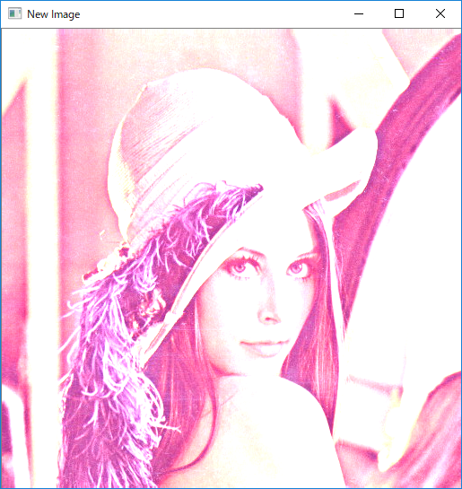
python\tutorial_code\Histograms_Matching\back_projection\calcBackProject_Demo1.py
python\tutorial_code\Histograms_Matching\back_projection\calcBackProject_Demo2.py
python\tutorial_code\Histograms_Matching\histogram_calculation\calcHist_Demo.py
python\tutorial_code\Histograms_Matching\histogram_comparison\compareHist_Demo.py
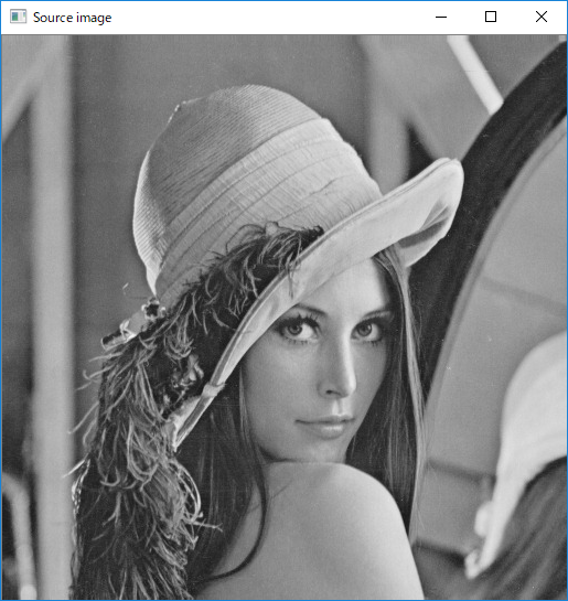
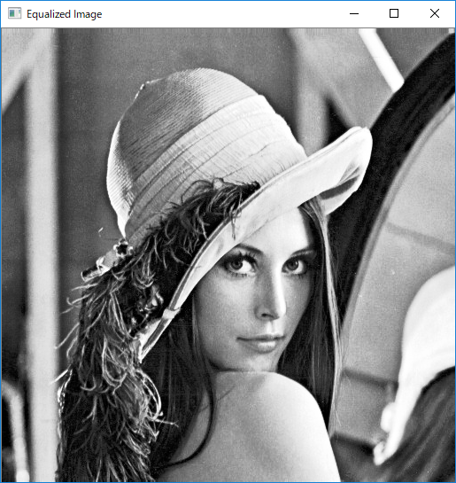
python\tutorial_code\Histograms_Matching\histogram_equalization\EqualizeHist_Demo.py
python\tutorial_code\imgProc\anisotropic_image_segmentation\anisotropic_image_segmentation.py
python\tutorial_code\imgProc\BasicGeometricDrawing\basic_geometric_drawing.py
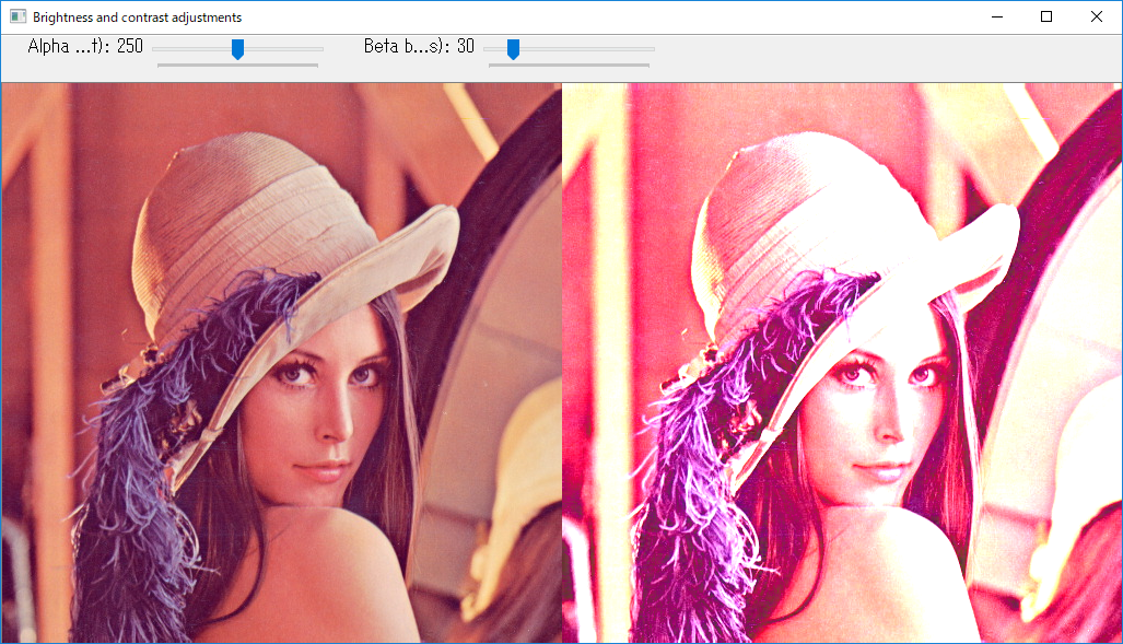
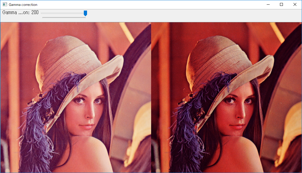
python\tutorial_code\imgProc\changing_contrast_brightness_image\BasicLinearTransforms.py

(py36) D:\python-opencv-sample\tutorial_code\imgProc\changing_contrast_brightness_image>python BasicLinearTransforms.py
 Basic Linear Transforms
-------------------------
* Enter the alpha value [1.0-3.0]: 2.0
* Enter the beta value [0-100]: 50
python\tutorial_code\imgProc\changing_contrast_brightness_image\changing_contrast_brightness_image.py
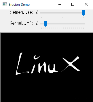
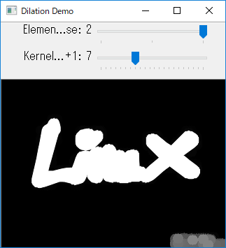
python\tutorial_code\imgProc\erosion_dilatation\morphology_1.py
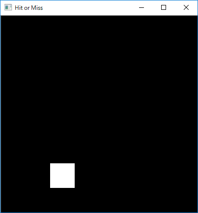
python\tutorial_code\imgProc\HitMiss\hit_miss.py
python\tutorial_code\imgProc\hough_line_transform\hough_line_transform.py
python\tutorial_code\imgProc\hough_line_transform\probabilistic_hough_line_transform.py
python\tutorial_code\imgProc\match_template\match_template.py
python\tutorial_code\imgProc\morph_lines_detection\morph_lines_detection.py
python\tutorial_code\imgProc\opening_closing_hats\morphology_2.py
python\tutorial_code\imgProc\Pyramids\pyramids.py
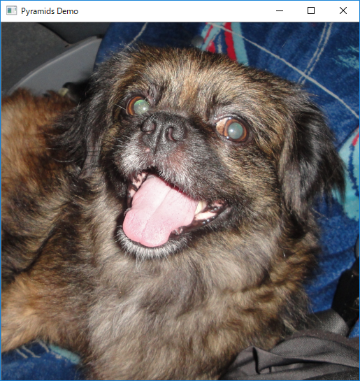
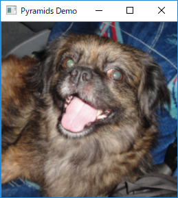
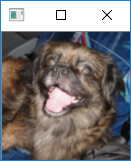
(py36) D:\python-opencv-sample\tutorial_code\imgProc\Pyramids>python pyramids.py

    Zoom In-Out demo
    ------------------
    * [i] -> Zoom [i]n
    * [o] -> Zoom [o]ut
    * [ESC] -> Close program

** Zoom In: Image x 2
** Zoom Out: Image / 2
** Zoom Out: Image / 2
** Zoom Out: Image / 2
python\tutorial_code\imgProc\Smoothing\smoothing.py
https://t.co/RkQbPgiD4x #OpenCV #Python pic.twitter.com/9xWiWDAOSz
— 藤本賢志(ガチ本)@くまもと復活祭/NT熊本/MF京都 (@sotongshi) April 10, 2019
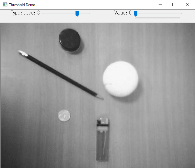
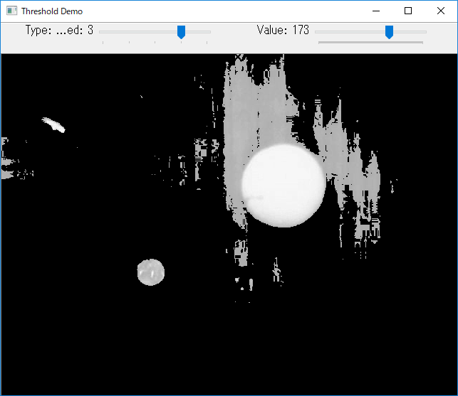
python\tutorial_code\imgProc\threshold\threshold.py
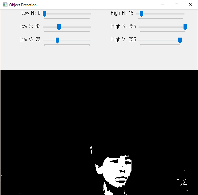
python\tutorial_code\imgProc\threshold_inRange\threshold_inRange.py
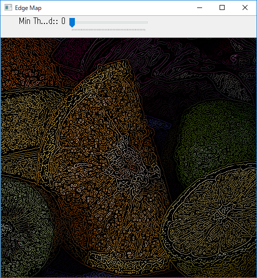
python\tutorial_code\ImgTrans\canny_detector\CannyDetector_Demo.py
python\tutorial_code\ImgTrans\distance_transformation\imageSegmentation.py
python\tutorial_code\ImgTrans\Filter2D\filter2D.py
https://t.co/jEojWil5jA #OpenCV #Python pic.twitter.com/TlEwAe34XN
— 藤本賢志(ガチ本)@くまもと復活祭/NT熊本/MF京都 (@sotongshi) April 10, 2019
python\tutorial_code\ImgTrans\HoughCircle\hough_circle.py
python\tutorial_code\ImgTrans\HoughLine\hough_lines.py
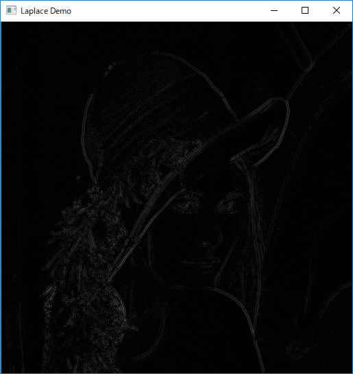
python\tutorial_code\ImgTrans\LaPlace\laplace_demo.py
python\tutorial_code\ImgTrans\MakeBorder\copy_make_border.py
copy_make_border.py #OpenCV #Python pic.twitter.com/RvpOwCKvkW
— 藤本賢志(ガチ本)@くまもと復活祭/NT熊本/MF京都 (@sotongshi) April 10, 2019
python\tutorial_code\ImgTrans\remap\Remap_Demo.py
Remap_Demo.py #OpenCV #Python pic.twitter.com/6EIrQuEyqR
— 藤本賢志(ガチ本)@くまもと復活祭/NT熊本/MF京都 (@sotongshi) April 10, 2019
python\tutorial_code\ImgTrans\SobelDemo\sobel_demo.py
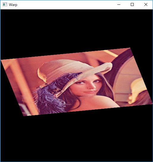
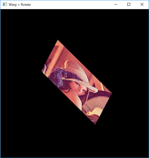
python\tutorial_code\ImgTrans\warp_affine\Geometric_Transforms_Demo.py

python\tutorial_code\introduction\documentation\documentation.py
(py36) D:\python-opencv-sample\tutorial_code\introduction\documentation>python documentation.py
Not showing this text because it is outside the snippet
Hello world!
python\tutorial_code\ml\introduction_to_pca\introduction_to_pca.py
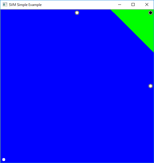
python\tutorial_code\ml\introduction_to_svm\introduction_to_svm.py
python\tutorial_code\ml\non_linear_svms\non_linear_svms.py
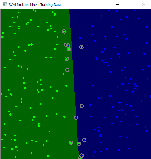
(py36) D:\python-opencv-sample\tutorial_code\ml\non_linear_svms>python non_linear_svms.py
Starting training process
Finished training process
python\tutorial_code\ml\py_svm_opencv\hogsvm.py
(py36) D:\python-opencv-sample\tutorial_code\ml\py_svm_opencv>python hogsvm.py
93.8
svm_data.datが生成される
python\tutorial_code\objectDetection\cascade_classifier\objectDetection.py
python\tutorial_code\photo\hdr_imaging\hdr_imaging.py
python\tutorial_code\ShapeDescriptors\bounding_rects_circles\generalContours_demo1.py
python\tutorial_code\ShapeDescriptors\bounding_rotated_ellipses\generalContours_demo2.py

python\tutorial_code\ShapeDescriptors\find_contours\findContours_demo.py
python\tutorial_code\ShapeDescriptors\hull\hull_demo.py

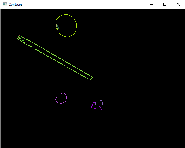
python\tutorial_code\ShapeDescriptors\moments\moments_demo.py

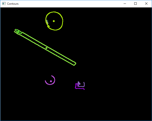
(py36) D:\python-opencv-sample\tutorial_code\ShapeDescriptors\moments>python moments_demo.py
 * Contour[0] - Area (M_00) = 9.00 - Area OpenCV: 9.00 - Length: 148.08
 * Contour[1] - Area (M_00) = 7.00 - Area OpenCV: 7.00 - Length: 140.77
 * Contour[2] - Area (M_00) = 23.50 - Area OpenCV: 23.50 - Length: 176.75
 * Contour[3] - Area (M_00) = 269.00 - Area OpenCV: 269.00 - Length: 1217.62
 * Contour[4] - Area (M_00) = 233.00 - Area OpenCV: 233.00 - Length: 80.91
 * Contour[5] - Area (M_00) = 207.50 - Area OpenCV: 207.50 - Length: 72.67
 * Contour[6] - Area (M_00) = 2.50 - Area OpenCV: 2.50 - Length: 35.56
 * Contour[7] - Area (M_00) = 3.00 - Area OpenCV: 3.00 - Length: 38.97
 * Contour[8] - Area (M_00) = 64.50 - Area OpenCV: 64.50 - Length: 511.63
python\tutorial_code\ShapeDescriptors\point_polygon_test\pointPolygonTest_demo.py
python\tutorial_code\TrackingMotion\corner_subpixels\cornerSubPix_Demo.py
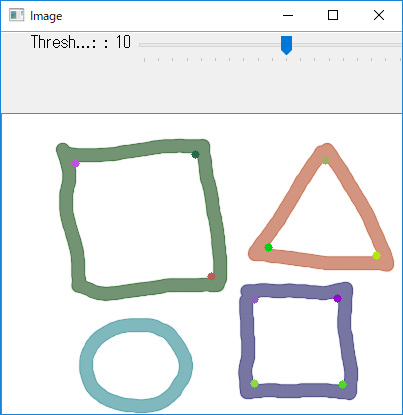
(py36) D:\python-opencv-sample\tutorial_code\TrackingMotion\corner_subpixels>python cornerSubPix_Demo.py
** Number of corners detected: 10
 -- Refined Corner [ 0 ]  ( 335.41644 , 182.86533 )
 -- Refined Corner [ 1 ]  ( 250.72044 , 183.83125 )
 -- Refined Corner [ 2 ]  ( 71.831924 , 47.796455 )
 -- Refined Corner [ 3 ]  ( 250.76755 , 269.47165 )
 -- Refined Corner [ 4 ]  ( 210.26521 , 163.34479 )
 -- Refined Corner [ 5 ]  ( 340.4781 , 270.57907 )
 -- Refined Corner [ 6 ]  ( 193.64813 , 38.78414 )
 -- Refined Corner [ 7 ]  ( 322.98306 , 45.351204 )
 -- Refined Corner [ 8 ]  ( 375.34808 , 141.40262 )
 -- Refined Corner [ 9 ]  ( 264.52493 , 133.20787 )
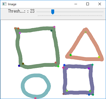
python\tutorial_code\TrackingMotion\generic_corner_detector\cornerDetector_Demo.py

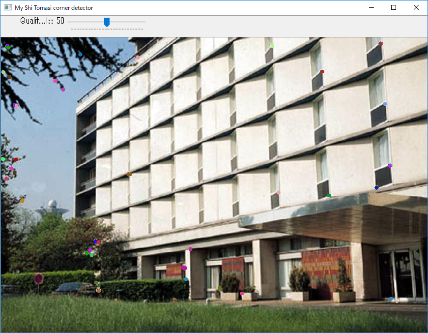
python\tutorial_code\TrackingMotion\good_features_to_track\goodFeaturesToTrack_Demo.py
(py36) D:\python-opencv-sample\tutorial_code\TrackingMotion\good_features_to_track>python goodFeaturesToTrack_Demo.py
** Number of corners detected: 23
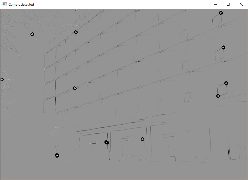
python\tutorial_code\TrackingMotion\harris_detector\cornerHarris_Demo.py
python\tutorial_code\video\background_subtraction\bg_sub.py
bg_sub.py #OpenCV #Python pic.twitter.com/8WM0wCTbYl
— 藤本賢志(ガチ本)@くまもと復活祭/NT熊本/MF京都 (@sotongshi) April 10, 2019