はじめに
植物が形作るパターンのひとつに、らせん型パターン(parastichy) があります。例えば、ひまわりの種の配置、松ぼっくりを上から見たときの傘の位置、多肉植物の葉の位置などがあります。

Sunflower,
Gardenkitty, CC BY-SA 3.0, ウィキメディア・コモンズ経由で

Spiral Aloe from above,
Sam, CC BY-SA 4.0, ウィキメディア・コモンズ経由で
これらのらせん型パターンの特徴はよく「フィボナッチ数列」や「黄金比」と関連させてやや神秘主義的に語られます。しかしながら、多くの場合、説明はそこまでで終わってしまい、「そのようならせん型パターンが、どのように形成されうるか」という"How"の部分にはあまり触れられません。この記事では、Douady and Couder[1]の論文をもとに動力学的な視点から提案されたパターン形成メカニズムを紹介します。
今回作るもの
考えるモデル
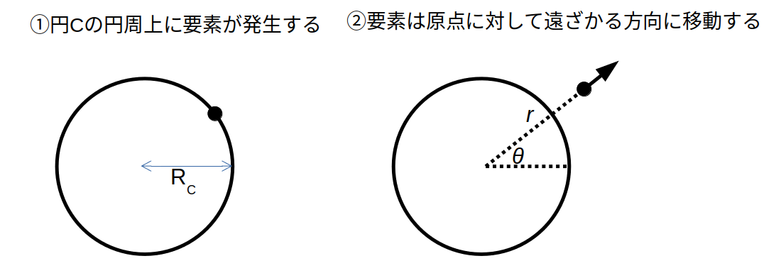
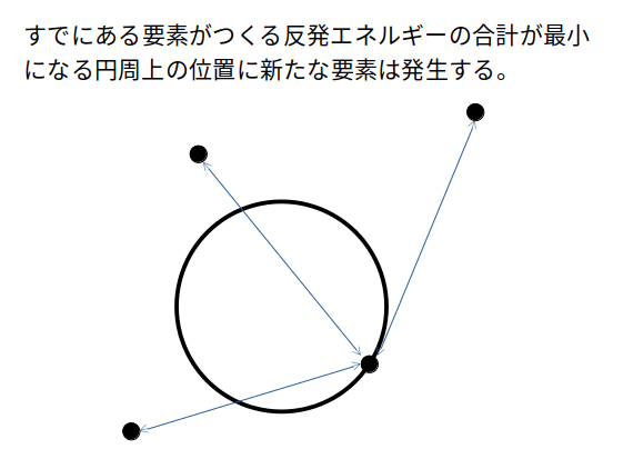
無限に広がる二次元平面を考えます。原点を中心に半径RC の円Cがあります。新しい種や葉(以下、要素と呼びます)はこの円の外縁において一定の周期 $T$ で発生します。発生した要素はある速度 $V$ で放射状に外側に移動していきます。各要素は反発エネルギーを生み出します。反発エネルギーの大きさは各要素間の距離 $d$ に反比例します。新しい要素は円C上において、すでに存在する要素がつくる反発エネルギーの合計が最小になる位置に発生します。
要素は円Cより外側では反発エネルギーの影響は受けません。すなわち要素自身が発生した瞬間の角度を維持しながら一定方向へ遠ざかっていきます。
このモデルは、植物において、新しい種や葉を生み出す組織が平面上に1つあり周期的に種や葉を生み出すプロセスをイメージしたものです。新しく生まれた種は後から生まれた種に押し出されてどんどん外側へと移動します。また、種はある程度の体積を持っているので新しい種は最も空いている空間に生み出されるとします。
植物との類似
| 植物 | 今回のモデル |
|---|---|
| 植物の種や葉(原基) | 大きさのない要素(粒子) |
| 種や葉のもととなる原基が発生する箇所(成長点) | 半径RCの円Cの周上 |
| 成長点から原基は比較的空いている空間に出てくる | 要素は円C外周上において反発エネルギー最小の位置に出現する |
| 原基は後から出現した原基に押されて外側に移動する | 要素は放射状に外側に移動する |
実験室実験
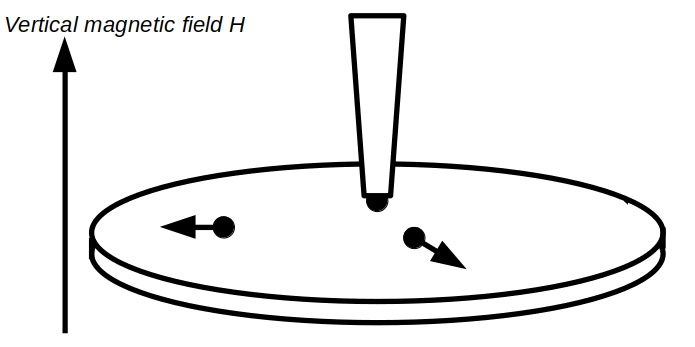
Douady and Couderら[2]は実験室で上述のモデルを再現しました。
まず、直径8cmの円盤をシリコンオイルで満たし垂直磁場中に置きます。垂直磁場は円盤中心から離れるほど強くなるようにします。円盤の中心にはビュレットのようなものをセットし、そこから一定の周期で磁性流体を滴下します。円盤上に落下した小滴は磁場によって分極し、互いに反発しあいます。これらの小滴は磁場の勾配によって外側に移動します。円盤の外周には溝があり、外縁に蓄積しないようにします(図では省略してあります)
実験の動画がYoutubeにあります。
小滴がらせん型のパターンをつくっているのが見て取れます。同じ実験を行うのは大変なのでコンピュータ上で実験を行いましょう。
数値計算によるシミュレーション
2次元平面の原点$O$を中心とする円があります。この円の半径は$R_0$であり円周上から新たな粒子(”要素”や”小滴”に相当)が生まれます。$i$番目の粒子の位置は極座標表示を用いて$(r_i,\theta_i)$と表されます。粒子は速度$V(r)$で放射状に移動します。速度は中心からの距離に依存します。
V(r)=\frac{V_0}{R_0} r
$V_0$は粒子の動きやすさを示すパラメータです。高いほど動きやすいです。実験室実験でいうとシリコンオイルの粘性や垂直磁場の強さに相当します。
粒子の発生間隔を$T$と置きます。
ここで
G=\frac{V_0 T}{R_0}
と定義される無次元パラメータ$G$を定義します。面白いことに、$V_0,T,R_0$によらず$G$が等しければ形成されるパターン(の選択肢)は同じになります。
たとえば
実験室実験でのスケール:$V_0$=1cm/sec, $T$=1sec, $R_0$=1cm
植物成長のスケール:$V_0$=0.001μm/sec, $T$=100000sec, $R_0$=100μm
では、どちらも$G$=1になり形成されるパターンは同じになります。この性質から、以降、無次元パラメータ$G$をふってシミュレーションを行います。
粒子は自身からの距離$d$に応じて反発エネルギーを生み出します。
E(d)=\frac{1}{d^3}
粒子$i$と粒子$j$との距離$d_{ij}$は余弦定理より
d_{ij}=\sqrt{r_i^2+r_j^2-2 r_i r_j \mathrm{cos}(\theta_j-\theta_i)}
です。円周上において、すでに平面上にある粒子たちの反発エネルギーの合計が最小になるところに新たな粒子は生成されます。
計算
計算はPython3を用い、VS Code上で実行しています。
最初にモジュールを読み込みします。
#計算用
import copy
import numpy as np
import scipy.optimize as opt

#描画用
from numpy.lib.function_base import vectorize
import matplotlib.pyplot as plt
import matplotlib.patches as patches
from matplotlib.animation import FuncAnimation
パラメータを設定します。ここではG=1です。
#%%
#パラメータ設定
velocity=0.5 #advection velocity,V
period=2 #period,T
time_step=0.01
radius=1.0 #radius of the circle outside which the angular postion of the particles is fixed
G=velocity*period/radius #relevant parameter
division_num=1800
Nmax=50
print(G)
計算します。時間刻みtime_stepごとに粒子の位置を更新し、発生周期を迎えたら反発エネルギー最小となる$\theta$を計算し、新たな粒子を追加します。ログはepisodeに保存しておきます。
#初期状態の定義
N=0 #number of particles
particles=np.array([[radius,0.0]]) #radius and angular of particles
next_ontogeny_timing=period

#エネルギー計算関数
def cost_function(theta,*args):
    particles=args[1]
    r=args[0]
    res=0

    for i in range(len(particles)):
        r2,theta2=particles[i,0],particles[i,1]
        dist=np.sqrt(r**2+r2**2-2.0*r*r2*np.cos(theta2-theta))
        res+=dist**-3

    return res

episode=[[[radius,0.0]]]

#計算
for i in range(1,int(Nmax*period/time_step)):
    t=time_step*i

    #時刻が粒子発生タイミングを追い抜いたとき
    if next_ontogeny_timing<=t-(1e-6):

        #反発エネルギー最小位置を求める(0.2°間隔で総当たり)
        energy_min_theta=opt.brute(cost_function,ranges=[(0,2*np.pi)],args=(radius,particles),Ns=division_num)

        #エネルギー最小の位置に粒子を一つ追加する
        new_particle=np.array([np.concatenate([np.array([radius]),energy_min_theta])])
        particles=np.append(particles,new_particle,axis=0)
        N+=1
        next_ontogeny_timing+=period

  #位置の更新
    for j in range(len(particles)):
        particles[j][0]+=velocity/radius*particles[j][0]*time_step

    episode.append(copy.copy(particles))
描画します。
#描画準備
#極座標から直交座標への変換
def polar_to_ortho_coord_x(r,theta):
    return r*np.cos(theta)

def polar_to_ortho_coord_y(r,theta):
    return r*np.sin(theta)

vectorized_polar_to_ortho_coord_x=vectorize(polar_to_ortho_coord_x)
vectorized_polar_to_ortho_coord_y=vectorize(polar_to_ortho_coord_y)

#描画
fig,axes=plt.subplots()
circle=patches.Circle(xy=(0,0),radius=radius,fill=False)
draw_interval=10

def animate(itr):
    step=itr*draw_interval
    particles_in_a_gen=np.array(episode[step])
    x=vectorized_polar_to_ortho_coord_x(particles_in_a_gen[:,0],particles_in_a_gen[:,1])
    y=vectorized_polar_to_ortho_coord_y(particles_in_a_gen[:,0],particles_in_a_gen[:,1])

    axes.cla()
    axes.add_patch(circle)
    axes.scatter(x,y,s=100)
    axes.set_xlim([-10,10])
    axes.set_ylim([-10,10])
    axes.set_aspect('equal')
    plt.title('spiral phyllotaxis, G={0:.2f} step={1:3d}'.format(G,step))

anim=FuncAnimation(fig,animate,frames=len(episode)//draw_interval)
anim.save("test_G=1.mp4", writer='ffmpeg',fps=6)
結果
G=1.0のとき
粒子が発生する間隔が長いとき、または発生した粒子がすぐに遠くに行ってしまうとき、1個前の粒子の反発エネルギーの影響のみが大きく$i$番目の粒子と$i+1$番目の粒子のなす角はつねに180°です。
Numerical simulation of spiral phyllotaxis, G=1.0, Ref:S.Douady and Y.Couder, J. theor. Biol. vol.178, 255-274(1996). pic.twitter.com/dlc6vyPSZZ
— STInverSpinel (@STInverSpinel) August 16, 2021
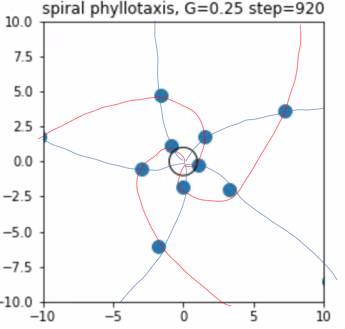
G=0.25のとき
実験室実験の動画(Youtube)の後半で見られたようなパターンが見られます。$i$番目の粒子と$i+1$番目の粒子のなす角は219.8°に収束しました。
Numerical simulation of spiral phyllotaxis, G=0.25, Ref:S.Douady and Y.Couder, J. theor. Biol. vol.178, 255-274(1996). pic.twitter.com/cKGbs5oo1P
— STInverSpinel (@STInverSpinel) August 16, 2021
(ちなみに、ここで形成されたパターンは下図のようにらせんに沿って線を引くと青い線が5本、赤い線が3本引けました。これを(3,5)らせんと呼びます。さきほどのG=1.0は(1,1)らせんです。$G$が0に近づくほど$(i,j)$らせんの$i,j$は増加します。$(i,j)$らせんが生じる値$G$が存在するとき、$G$を少しずつ下げていくとある値から$(i,i+j)$と$(j,i+j)$らせんに分岐します。ここらへんがフィボナッチ数列やリュカ数列とからんできます。詳しいことを知りたい方は元論文[1]をご覧ください。)
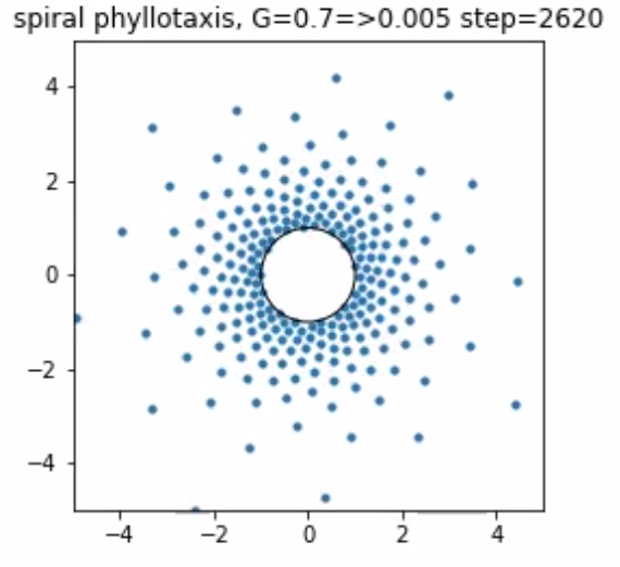
Gを急激に減少させたとき
Numerical simulation of spiral phyllotaxis, Ref:S.Douady and Y.Couder, "Phyllotaxis as a dynamical self organizing process part I: The spiral modes resulting from time-periodic iterations", J. theor. Biol. vol.178, 255-274(1996). pic.twitter.com/wvis27XDVr
— STInverSpinel (@STInverSpinel) August 16, 2021
#%%
import time
import numpy as np
import scipy.optimize as opt
import copy
import matplotlib.pyplot as plt
import matplotlib.patches as patches
from numpy.lib.function_base import vectorize
from matplotlib.animation import FuncAnimation

#%%
#パラメータ設定
velocity=0.5 #advection velocity,V
period=1.4 #period,T
time_step=0.01
radius=1.0 #radius of the circle outside which the angular postion of the particles is fixed
G=velocity*period/radius #relevant parameter
Nmax=300
print(G)
lower_limit_T=0.01
cooling_rate=0.94

#%%
#初期状態の定義
N=0 #number of particles
particles=np.array([[radius,0.0]]) #radius and angular of particles
next_ontogeny_timing=period

#エネルギー計算関数
def cost_function(theta,*args):
    particles=args[1]
    r=args[0]
    res=0

    for i in range(len(particles)-1,-1,-1):
        r2,theta2=particles[i,0],particles[i,1]
        dist=np.sqrt(r**2+r2**2-2.0*r*r2*np.cos(theta2-theta))

        res+=dist**-3

    return res

vectorized_update_pos=np.vectorize(update_positions)

episode=[[[radius,0.0]]]

#時間計測開始
time_start=time.time()
print("start")

for i in range(1,int(Nmax*period/time_step)):
    t=time_step*i

    #時刻が粒子発生タイミングを追い抜いたとき
    if next_ontogeny_timing<=t-(1e-6):

        #反発エネルギー最小位置を求める
        division_num=1800

        energy_min_theta=opt.brute(cost_function,ranges=[(0,2*np.pi)],args=(radius,particles),Ns=division_num)

        #要素を一つ追加する
        new_particle=np.array([np.concatenate([np.array([radius]),energy_min_theta])])
        particles=np.append(particles,new_particle,axis=0)
        N+=1
        period=period*cooling_rate
        next_ontogeny_timing+=period+lower_limit_T

    if Nmax<=N:
        break

    #位置の更新
    #particles[:,0]=vectorized_update_pos(particles[:,0])

    for j in range(len(particles)):
        #print(particles[j][0])
        particles[j][0]+=velocity/radius*particles[j][0]*time_step

    episode.append(copy.copy(particles))

time_end=time.time()
time_per=time_end-time_start
print("end")
print(time_per)

#%%
#描画準備
#極座標から直交座標への変換
def polar_to_ortho_coord_x(r,theta):
    return r*np.cos(theta)

def polar_to_ortho_coord_y(r,theta):
    return r*np.sin(theta)

vectorized_polar_to_ortho_coord_x=vectorize(polar_to_ortho_coord_x)
vectorized_polar_to_ortho_coord_y=vectorize(polar_to_ortho_coord_y)

#描画
fig,axes=plt.subplots()
circle=patches.Circle(xy=(0,0),radius=radius,fill=False)
draw_interval=10

def animate(itr):
    step=itr*draw_interval
    particles_in_a_gen=np.array(episode[step])
    x=vectorized_polar_to_ortho_coord_x(particles_in_a_gen[:,0],particles_in_a_gen[:,1])
    y=vectorized_polar_to_ortho_coord_y(particles_in_a_gen[:,0],particles_in_a_gen[:,1])

    axes.cla()
    axes.add_patch(circle)
    axes.scatter(x,y,s=10)
    limit=5
    axes.set_xlim([-limit,limit])
    axes.set_ylim([-limit,limit])
    axes.set_aspect('equal')
    plt.title('spiral phyllotaxis, G=0.7=>0.005 step={0:3d}'.format(step))

anim=FuncAnimation(fig,animate,frames=len(episode)//draw_interval)
anim.save("test_sunflower.mp4", writer='ffmpeg',fps=8)
結論と感想
「反発エネルギーが最小となる位置に粒子をつくる」という簡単なモデルでも、複雑ならせん型パターンを作ることができました。
ただし、らせん型パターンが作れたからといってこのモデルと同様な機構が植物に存在するとは必ずしも言い切れません。しかしながら、遺伝学的に「植物の遺伝子にフィボナッチ数列が埋め込まれている」と考えるよりは、この記事で述べたような物理学的機構がパターン形成に関わっていると考えるほうがありえそうに思います。
参考文献
[1]S.Douady and Y.Couder, "Phyllotaxis as a dynamical self organizing process part I: The spiral modes resulting from time-periodic iterations", J. theor. Biol. vol.178, 255-274(1996).
[2]S.Douady and Y.Couder, "Phyllotaxis as self organised growth process", Phys. Rev. Lett vol.68, 2098-2101(1992).