はじめに
@piacerex さんから、以下のポストを紹介していただきました
Elixir の Nx で線形回帰を実装した記事があったので、これを参考に 4PL を実装してみました
4PL では、以下の数式で表される曲線の A, B, C, D のパラメータを調整していきます
f(x) = \frac{A-D}{1+(x/C)^B}+ D
実装環境は Livebook です
実装したノートブックはこちら
必要なモジュールのインストール
Nx など、必要なモジュールをインストールします
Mix.install([
  {:nx, "~> 0.7"},
  {:exla, "~> 0.7"},
  {:kino, "~> 0.12"},
  {:kino_vega_lite, "~> 0.1"},
  {:statistics, "~> 0.6"}
])

Nx.global_default_backend(EXLA.Backend)
Statistics は正規分布の乱数をノイズとして発生させるために使用します
データ準備
Python の 4PL 実装例を参考に、まずは元となるデータを作成します
X は 0 から 19 の整数とします
x_data = Nx.iota({20})
実行結果
#Nx.Tensor<
  s64[20]
  EXLA.Backend<host:0, 0.3354478297.604635146.93493>
  [0, 1, 2, 3, 4, 5, 6, 7, 8, 9, 10, 11, 12, 13, 14, 15, 16, 17, 18, 19]
>
今回は正解とする各パラメータを A=0.5, B=2.5, C= 8, D=7.3 とします
f(x) = \frac{A-D}{1+(x/C)^B}+ D
そのため、 X に対する Y の値(正解の曲線上にある値)を以下のように生成します
true_y_data =
  Nx.divide(
    0.5-7.3,
    Nx.divide(x_data, 8)
    |> Nx.pow(2.5)
    |> Nx.add(1)
  )
  |> Nx.add(7.3)
実行結果
#Nx.Tensor<
  f32[20]
  EXLA.Backend<host:0, 0.3354478297.605421578.13981>
  [0.5, 0.5373587608337402, 0.7060604095458984, 1.0391521453857422, 1.5215034484863281, 2.1044654846191406, 2.7274622917175293, 3.3377039432525635, 3.9000000953674316, 4.3969926834106445, 4.824507713317871, 5.186199188232422, 5.489407539367676, 5.7425642013549805, 5.953813552856445, 6.1304030418396, 6.278496742248535, 6.403209686279297, 6.508727550506592, 6.598447799682617]
>
観測値を想定し、曲線の値に対してノイズを加えます
y_data =
  true_y_data
  |> Nx.add(
    1..20
    |> Enum.map(fn _ -> Statistics.Distributions.Normal.rand() end)
    |> Nx.tensor()
    |> Nx.multiply(0.2)
  )
実行結果
#Nx.Tensor<
  f32[20]
  EXLA.Backend<host:0, 0.3354478297.605421578.13983>
  [0.29586589336395264, 0.6543958783149719, 1.087601661682129, 1.0075170993804932, 1.6051973104476929, 1.9136173725128174, 2.723944902420044, 3.596914052963257, 4.239219665527344, 4.431465148925781, 4.693841457366943, 5.0326948165893555, 5.504952430725098, 5.711021423339844, 5.865734577178955, 5.940439224243164, 6.16650390625, 6.853420734405518, 6.261311054229736, 6.689829349517822]
>
正解となる曲線とノイズを加えた値をグラフ化します
plot_data =
  %{
    x: x_data |> Nx.to_flat_list(),
    y: y_data |> Nx.to_flat_list()
  }

true_plot_data =
  %{
    x: x_data |> Nx.to_flat_list(),
    y: true_y_data |> Nx.to_flat_list()
  }

VegaLite.new(width: 600)
|> VegaLite.layers([
  VegaLite.new()
  |> VegaLite.data_from_values(plot_data)
  |> VegaLite.mark(:point)
  |> VegaLite.encode_field(:x, "x", type: :quantitative)
  |> VegaLite.encode_field(:y, "y", type: :quantitative),
  VegaLite.new()
  |> VegaLite.data_from_values(true_plot_data)
  |> VegaLite.mark(:line, color: "#ff0000")
  |> VegaLite.encode_field(:x, "x", type: :quantitative)
  |> VegaLite.encode_field(:y, "y", type: :quantitative)
])
|> Kino.VegaLite.new()

トレーニング
4PL 用のモジュールを作成します
defmodule FPL do
  import Nx.Defn

  defn pred({a, b, c, d}, x) do
    (a - d) / (1.0 + Nx.pow(x / c, b)) + d
  end

  defn mse(yp, y) do
    (yp - y)
    |> Nx.pow(2)
    |> Nx.mean()
  end

  defn loss(params, x, y) do
    yp = pred(params, x)
    mse(yp, y)
  end

  defn update({a, b, c, d} = params, x, y, lr) do
    {grad_a, grad_b, grad_c, grad_d} = grad(params, &loss(&1, x, y))
    {
      a - grad_a * lr,
      b - grad_b * lr,
      c - grad_c * lr,
      d - grad_d * lr
    }
  end

  defn init_params do
    {Nx.tensor(1.0), Nx.tensor(1.0), Nx.tensor(1.0), Nx.tensor(1.0)}
  end

  def loss_update({lvs, a, b, c, d}, x, y, lr) do
    lv = FPL.loss({a, b, c, d}, x, y)
    {a, b, c, d} = FPL.update({a, b, c, d}, x, y, lr)
    {[Nx.to_number(lv) | lvs], a, b, c, d}
  end
end
線形回帰の実装から pred の関数と各関数のパラメータを変更しただけです
学習時の損失と回帰曲線を表示するためのグラフを用意します
loss_widget =
  VegaLite.new(width: 600)
  |> VegaLite.mark(:line)
  |> VegaLite.encode_field(:x, "x", type: :quantitative, title: "epoch")
  |> VegaLite.encode_field(:y, "y", type: :quantitative, title: "loss")
  |> Kino.VegaLite.new()

fpl_widget =
  VegaLite.new(width: 600)
  |> VegaLite.layers([
    VegaLite.new()
    |> VegaLite.data_from_values(plot_data)
    |> VegaLite.mark(:point)
    |> VegaLite.encode_field(:x, "x", type: :quantitative)
    |> VegaLite.encode_field(:y, "y", type: :quantitative),
    VegaLite.new()
    |> VegaLite.data_from_values(true_plot_data)
    |> VegaLite.mark(:line, color: "#ff0000")
    |> VegaLite.encode_field(:x, "x", type: :quantitative)
    |> VegaLite.encode_field(:y, "y", type: :quantitative),
    VegaLite.new()
    |> VegaLite.mark(:line)
    |> VegaLite.encode_field(:x, "x", type: :quantitative)
    |> VegaLite.encode_field(:y, "y", type: :quantitative)
  ])
  |> Kino.VegaLite.new()

Kino.VegaLite.clear(loss_widget)
Kino.VegaLite.clear(fpl_widget)

Kino.Layout.grid([loss_widget, fpl_widget], columns: 1)
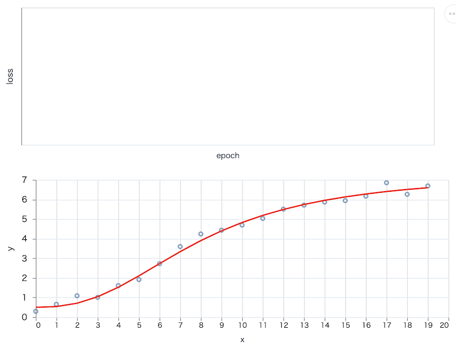
各グラフには以下のデータを表示します
- 上のグラフ: トレーニングの各エポック時点での損失(この時点では空)
- 下のグラフ: 現時点で調整したパラメータによる回帰曲線(この時点では観測値と正解の曲線のみ)
グラフを更新するための関数を用意します
update_plots = fn {epoch, lvs, a, b, c, d} ->
  loss_plot_data =
    1..epoch
    |> Enum.zip(Enum.reverse(lvs))
    |> Enum.map(fn {x, y} -> %{x: x, y: y} end)

  Kino.VegaLite.clear(loss_widget)
  Kino.VegaLite.push_many(loss_widget, loss_plot_data)

  yl_data = FPL.pred({a, b, c, d}, x_data)
  fpl_plot_data =
    Enum.zip(
      x_data |> Nx.to_flat_list(),
      yl_data |> Nx.to_flat_list()
    )
    |> Enum.map(fn {x, y} -> %{x: x, y: y} end)

  Kino.VegaLite.clear(fpl_widget)
  Kino.VegaLite.push_many(fpl_widget, fpl_plot_data)
end
トレーニングを実行します
# 初期値
{a, b, c, d} = FPL.init_params()

# エポック数
epochs = 2500

# 学習率
lr = 0.02

Enum.reduce(1..epochs, {[], a, b, c, d}, fn epoch, acc ->
  {lvs, a, b, c, d} = FPL.loss_update(acc, x_data, y_data, lr)

  # 10 エポックに 1 回グラフを更新する
  if rem(epoch, 10) == 0 do
    update_plots.({epoch, lvs, a, b, c, d})
  end

  {lvs, a, b, c, d}
end)
実行すると、用意しておいたグラフがリアルタイムに更新されます
エポックが進むと正解の曲線(赤いグラフ)に対して推測した曲線(青いグラフ)がどんどんフィットしているのが分かります

実行結果
{[0.0438070073723793, 0.043814517557621, 0.043822031468153, 0.043829597532749176, ...],
 #Nx.Tensor<
   f32
   EXLA.Backend<host:0, 0.3354478297.605421578.139135>
   0.49458378553390503
 >,
 #Nx.Tensor<
   f32
   EXLA.Backend<host:0, 0.3354478297.605421578.139147>
   2.624643325805664
 >,
 #Nx.Tensor<
   f32
   EXLA.Backend<host:0, 0.3354478297.605421578.139160>
   7.424412250518799
 >,
 #Nx.Tensor<
   f32
   EXLA.Backend<host:0, 0.3354478297.605421578.139165>
   6.954604625701904
 >}
正解と推測のパラメータについて、かなり近いことがわかります
| パラメータ | 正解 | 推測 |
|---|---|---|
| A | 0.5 | 0.49 |
| B | 2.5 | 2.62 |
| C | 8.0 | 7.42 |
| D | 7.3 | 6.95 |
まとめ
Nx を使って 4PL が実装できました
関数さえ変えれば他の曲線も実装できそうです