More than 1 year has passed since last update.

株式会社オーイーシー

Elixir Axon で MNIST （手書き数字）の画像分類モデルをトレーニングする

Last updated at 2023-08-09Posted at 2023-08-09

はじめに

Livebook で画像分類モデルのトレーニングを実行します

内容は Axon 公式ドキュメントの "Classifying handwritten digits" = 「手書き数字の分類」に沿っています

すでに @the_haigo さん、 @sand さん、 @piacerex さんが記事を書いているので後発ですが、 Livebook ならではの視覚化要素を加えます

逆にこちらでは機械学習の詳細は解説しません

実装したノートブックはこちら

Google Colaboratory での Livebook の起動

機械学習のトレーニングは非常に重い処理なので、やはり GPU が使いたいですね

以下の記事を参考に、 Google Colaboratory 上で Livebook を起動します

セットアップ

Mix.install(
  [
    {:axon, "~> 0.5"},
    {:nx, "~> 0.5"},
    {:exla, "~> 0.5"},
    {:req, "~> 0.3"},
    {:kino, "~> 0.10"},
    {:kino_vega_lite, "~> 0.1"}
  ],
  config: [
    nx: [default_backend: EXLA.Backend]
  ],
  system_env: [
    {"XLA_TARGET", "cuda118"},
    {"EXLA_TARGET", "cuda"}
  ]
)

各パッケージの最新版をインストールします

Livebook 上で画像を表示したいので、 Kino もインストールしています

グラフを使いたいので KinoVegaLite もインストールします

また、 EXLA で GPU を使う設定を入れています

データのダウンロード

MNIST の画像と、その画像が表す数字（ラベル）のデータをダウンロードします

base_url = "https://storage.googleapis.com/cvdf-datasets/mnist/"
%{body: train_images} = Req.get!(base_url <> "train-images-idx3-ubyte.gz")
%{body: train_labels} = Req.get!(base_url <> "train-labels-idx1-ubyte.gz")

バイナリデータなのでそのままだと読めません

先頭のヘッダー情報を取得すると、画像枚数や画像サイズを取得することができます

<<_::32, n_images::32, n_rows::32, n_cols::32, images::binary>> = train_images

{n_images, n_rows, n_cols}

結果は {60000, 28, 28} となり、縦 28 ピクセル x 横 28 ピクセルの画像が 60,000 枚含まれている、ということが分かります

ラベルデータも同様にヘッダーから画像枚数を取得します

<<_::32, n_labels::32, labels::binary>> = train_labels

n_labels

結果は 60000 で、画像と同じ数のラベルが格納されています

データの変換

機械学習用にデータを変換します

images_tensor =
  images
  |> Nx.from_binary(:u8)
  |> Nx.reshape(
    {n_images, 1, n_rows, n_cols},
    names: [:images, :channels, :height, :width]
  )

Nx.from_binary(:u8) で、データを 8 ビット毎の符号なし整数（0 〜 255）として読み込みます

ヘッダ情報から取得した情報を元に、このデータを 60,000 x 1 x 28 x 28 の形に変換します

結果は以下のようになります

#Nx.Tensor<
  u8[images: 60000][channels: 1][height: 28][width: 28]
  EXLA.Backend<cuda:0, 0.1402569673.3419537415.33072>
  [
    [
      [
        [0, 0, 0, 0, 0, 0, 0, 0, 0, 0, 0, 0, 0, 0, 0, 0, 0, 0, 0, 0, 0, 0, 0, 0, 0, 0, 0, 0],
        [0, 0, 0, 0, 0, 0, 0, 0, 0, 0, 0, 0, 0, 0, 0, 0, 0, 0, 0, 0, 0, 0, ...],
        ...
      ]
    ],
    ...
  ]
>

テンソルの各次元は以下を意味します

:images: 画像枚数
:channels が色（白黒画像なので 1、カラーの場合は 3）
:height が画像の高さ = 縦ピクセル数
:width が画像の幅 = 横ピクセル数

このままだと、どういうデータなのか分かりにくいため、画像として表示してみます

images_display =
  images_tensor
  # 画像 1 枚毎に分割
  |> Nx.to_batched(1)
  # 先頭100枚
  |> Enum.slice(0..99)
  # 画像毎に形式を変換して表示
  |> Enum.map(fn tensor ->
    tensor
    # 画像枚数の次元を削減する
    |> Nx.squeeze(axes: [:images])
    # 色、高さ、幅を高さ、幅、色の順に変える
    |> Nx.transpose(axes: [:height, :width, :channels])
    |> Kino.Image.new()
  end)

# 10列に並べて表示
Kino.Layout.grid(images_display, columns: 10)

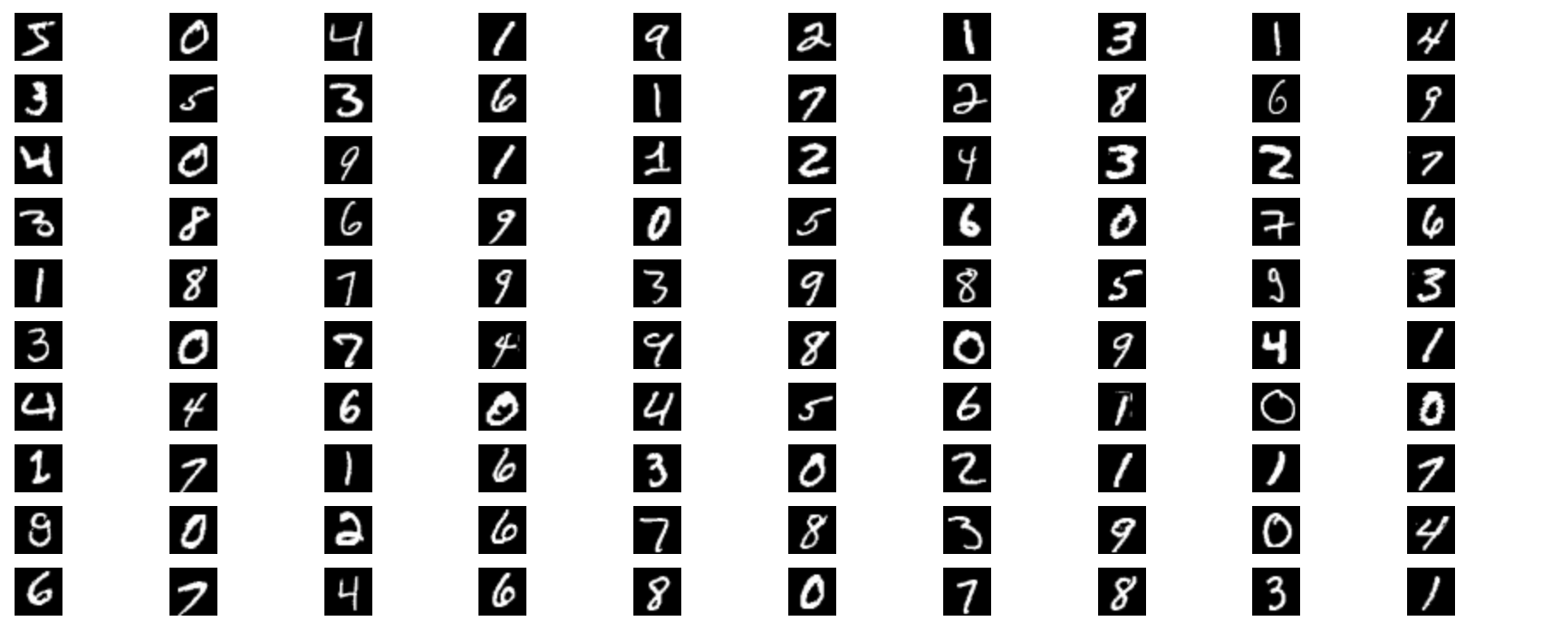
白黒画像の手書き数字になっていることが分かります

ラベルデータも同様にテンソルとして読み込みます

labels_tensor = Nx.from_binary(labels, :u8)

結果は以下の通りです

#Nx.Tensor<
  u8[60000]
  EXLA.Backend<cuda:0, 0.1402569673.3419537415.33558>
  [5, 0, 4, 1, 9, 2, 1, 3, 1, 4, 3, 5, 3, 6, 1, 7, 2, 8, 6, 9, 4, 0, 9, 1, 1, 2, 4, 3, 2, 7, 3, 8, 6, 9, 0, 5, 6, 0, 7, 6, 1, 8, 7, 9, 3, 9, 8, 5, 9, 3, ...]
>

5, 0, 4, ... という値が、画像に手書きされた数字を示すラベルになっています

画像と同じように並べてみましょう

labels_display =
  labels_tensor
  |> Nx.to_batched(1)
  |> Enum.slice(0..99)
  |> Enum.map(fn tensor ->
    tensor
    |> Nx.squeeze()
    |> Nx.to_number()
    |> Integer.to_string()
    |> Kino.Markdown.new()
  end)

Kino.Layout.grid(labels_display, columns: 10)

せっかくなので画像と並べてみましょう

images_display
|> Enum.zip(labels_display)
|> Enum.map(fn {image, label} ->
  Kino.Layout.grid([image, label], columns: 2)
end)
|> Kino.Layout.grid(columns: 10)

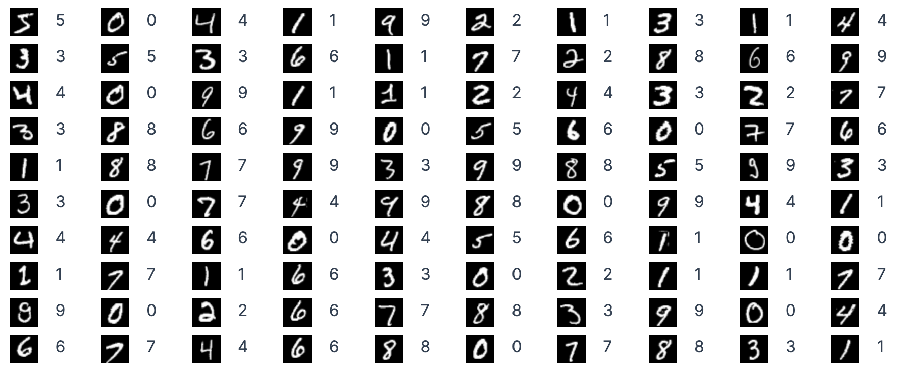
画像とラベルが一致していますね

バッチサイズ = トレーニング時に一度に読み込む画像枚数を指定します

batch_size = 32

画像データの各ピクセル値は 0 〜 255 の整数になっているので、これを 0 〜 1 の浮動小数に変換し、 32 枚毎のバッチに分割します

images_input =
  images_tensor
  |> Nx.divide(255)
  |> Nx.to_batched(batch_size)

ラベルデータは大きさではなくカテゴリなので、 one-hot エンコーディングします

例えば 5 は [0, 0, 0, 0, 0, 1, 0, 0, 0, 0] （index = 5 のところだけ 1）になります

labels_input =
  labels_tensor
  |> Nx.new_axis(-1)
  |> Nx.equal(Nx.tensor(Enum.to_list(0..9)))

結果は以下のようになります

#Nx.Tensor<
  u8[60000][10]
  EXLA.Backend<cuda:0, 0.1402569673.3420061703.75553>
  [
    [0, 0, 0, 0, 0, 1, 0, 0, 0, 0],
    [1, 0, 0, 0, 0, 0, 0, 0, 0, 0],
    [0, 0, 0, 0, 1, 0, 0, 0, 0, 0],
    [0, 1, 0, 0, 0, 0, 0, 0, 0, 0],
    [0, 0, 0, 0, 0, 0, 0, 0, 0, 1],
    ...
  ]
>

以下のようにちゃんと one-hot になっています

5 = [0, 0, 0, 0, 0, 1, 0, 0, 0, 0]
0 = [1, 0, 0, 0, 0, 0, 0, 0, 0, 0]
4 = [0, 0, 0, 0, 1, 0, 0, 0, 0, 0]

こちらもバッチに分割します

labels_input = Nx.to_batched(labels_input, batch_size)

モデルの定義

ニューラルネットワークの層を定義します

model =
  Axon.input("input", shape: {nil, 1, n_rows, n_cols})
  |> Axon.flatten()
  |> Axon.dense(128, activation: :relu)
  |> Axon.dense(10, activation: :softmax)

入力層は {nil, 1, n_rows, n_cols} の形式で入力できるようにします

画像枚数は nil なので任意の枚数、色は白黒なので 1 、高さと幅は MNIST の画像サイズと同じにします

中間層（隠れ層）では ReLu 関数を指定します

出力層では 10 カテゴリ（10種類の数字）に分類し、 softmax 関数でカテゴリ毎の確率（合計 1）に変換します

トレーニングの実行

トレーニングを実行します

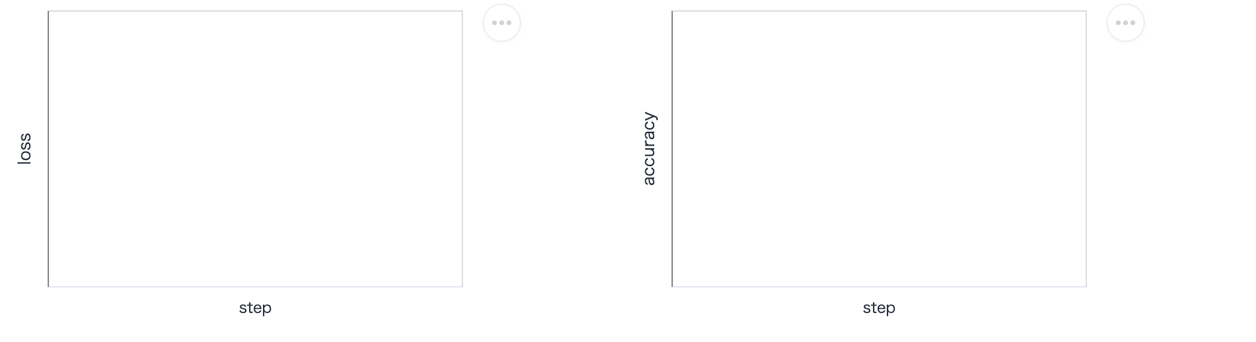
まず、トレーニング中の正解率やロスをグラフ表示するための枠を準備します

loss_plot =
  VegaLite.new(width: 300)
  |> VegaLite.mark(:line)
  |> VegaLite.encode_field(:x, "step", type: :quantitative)
  |> VegaLite.encode_field(:y, "loss", type: :quantitative)
  |> Kino.VegaLite.new()

acc_plot =
  VegaLite.new(width: 300)
  |> VegaLite.mark(:line)
  |> VegaLite.encode_field(:x, "step", type: :quantitative)
  |> VegaLite.encode_field(:y, "accuracy", type: :quantitative)
  |> Kino.VegaLite.new()

Kino.Layout.grid([loss_plot, acc_plot], columns: 2)

トレーニング用の設定をして、トレーニングを開始します

params =
  model
  # 損失関数と最適化関数を指定
  |> Axon.Loop.trainer(:categorical_cross_entropy, :adam)
  # 正解率をデバッグ表示
  |> Axon.Loop.metric(:accuracy, "accuracy")
  # グラフ表示
  |> Axon.Loop.kino_vega_lite_plot(loss_plot, "loss", event: :epoch_completed)
  |> Axon.Loop.kino_vega_lite_plot(acc_plot, "accuracy", event: :epoch_completed)
  # 入力、最大エポック数を指定してトレーニング実行
  |> Axon.Loop.run(Stream.zip(images_input, labels_input), %{}, epochs: 10, compiler: EXLA)

学習状況はエポック毎に表示されていきます

04:11:22.083 [debug] Forwarding options: [compiler: EXLA] to JIT compiler
Epoch: 0, Batch: 1850, Accuracy: 0.9240163 loss: 0.2673235
Epoch: 1, Batch: 1825, Accuracy: 0.9648725 loss: 0.1933463
Epoch: 2, Batch: 1850, Accuracy: 0.9764208 loss: 0.1546099
Epoch: 3, Batch: 1825, Accuracy: 0.9828407 loss: 0.1306373
Epoch: 4, Batch: 1850, Accuracy: 0.9873450 loss: 0.1127186
Epoch: 5, Batch: 1825, Accuracy: 0.9910548 loss: 0.0993479
Epoch: 6, Batch: 1850, Accuracy: 0.9936416 loss: 0.0884454
Epoch: 7, Batch: 1825, Accuracy: 0.9954354 loss: 0.0798224
Epoch: 8, Batch: 1850, Accuracy: 0.9960552 loss: 0.0724808
Epoch: 9, Batch: 1825, Accuracy: 0.9966508 loss: 0.0665720

また、グラフはエポック単位で更新されます

正解率は 0.924 から 0.997 まで上昇しています

ロスは 0.267 から 0.067 まで下降しています

問題なくトレーニングできているようです

予測

トレーニング結果のパラメータを使って予測してみましょう

バッチの先頭データ（32枚の画像）をモデルに渡して結果を取得します

first_batch = Enum.at(images_input, 0)

output = Axon.predict(model, params, first_batch)

出力結果は以下のようになります

#Nx.Tensor<
  f32[32][10]
  EXLA.Backend<cuda:0, 0.1402569673.3420061702.12190>
  [
    [2.1990186225590232e-20, 9.818139357076205e-11, 8.541999746425333e-11, 0.07378459721803665, 4.16927039994179e-25, 0.926215410232544, 4.593698357379851e-22, 4.2708387824538785e-13, 3.066993477219247e-14, 1.3510484397905032e-11],
    [0.9999996423721313, 8.137790160802477e-16, 3.220991118269012e-7, 4.544926379148294e-14, 1.94321618902048e-15, 2.8232578831743384e-14, 8.393934852746199e-12, 1.1132140131583923e-12, 1.6966183435918568e-14, 4.4457319769986015e-12],
    [3.4515617031161128e-9, 5.959921001164048e-9, 2.870689786504954e-5, 5.813278747268669e-10, 0.9999550580978394, 7.443362766423878e-12, 4.950033982709101e-8, 9.435645438315987e-7, 1.068484607458231e-7, 1.508475725131575e-5],
    [3.3670323473788955e-12, 0.9999990463256836, 2.536882846015942e-7, 2.017576106183583e-9, 1.9305321785623164e-8, 2.733279991229409e-10, 1.5964944210383747e-12, 5.806140848108043e-7, 7.061674267561102e-8, 6.687658426037446e-15],
    [2.67465194930714e-17, 3.61318810428949e-14, 1.2676755478668866e-11, 2.690524247839221e-9, 9.246244189853314e-6, 3.20018421484658e-11, 9.545354076132232e-18, 2.2851216474606417e-9, 9.275893120275214e-8, 0.999990701675415],
    ...
  ]
>

32 枚の画像 x 10 カテゴリ毎の確率がテンソルとして返っています

このままだと分かりにくいので、結果を整形します

まず、各画像毎に確率が最も高いカテゴリを予測ラベルとして取得します

predicted_labels =
  output
  |> Nx.argmax(axis: 1)
  |> Nx.to_flat_list()

結果は以下のようになります

[5, 0, 4, 1, 9, 2, 1, 3, 1, 4, 3, 5, 3, 6, 1, 7, 2, 8, 6, 9, 4, 0, 9, 1, 3, 2, 4, 3, 2, 7, 3, 8]

また、各画像毎に最も高い確率が予測ラベルに対する確信度です

scores =
  output
  |> Nx.reduce_max(axes: [1])
  |> Nx.to_flat_list()

結果は以下の通りです

[0.926215410232544, 0.9999996423721313, 0.9999550580978394, 0.9999990463256836, 0.999990701675415,
 0.9999986886978149, 0.9999936819076538, 1.0, 0.9998071193695068, 1.0, 1.0, 0.999997615814209, 1.0,
 0.9999997615814209, 0.99974125623703, 1.0, 0.9999992847442627, 0.9999997615814209,
 0.9884675145149231, 0.9999128580093384, 1.0, 0.9999986886978149, 0.9999562501907349,
 0.9999997615814209, 0.704083263874054, 0.9999867677688599, 0.9999992847442627, 1.0,
 0.999995231628418, 0.9952540993690491, 0.9992020726203918, 0.9998855590820312]

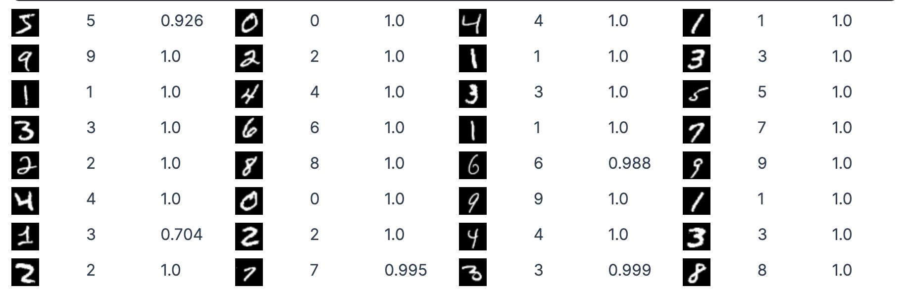
入力画像と予測ラベル、確信度を並べて表示します

[
  Nx.to_batched(first_batch, 1),
  predicted_labels,
  scores
]
|> Enum.zip()
|> Enum.map(fn {tensor, predicted_label, score} ->
  [
    tensor
    |> Nx.multiply(255)
    |> Nx.as_type(:u8)
    |> Nx.squeeze(axes: [0])
    |> Nx.transpose(axes: [1, 2, 0])
    |> Kino.Image.new(),
    predicted_label
    |> Integer.to_string()
    |> Kino.Markdown.new(),
    score
    |> Float.round(3)
    |> Float.to_string()
    |> Kino.Markdown.new()
  ]
  |> Kino.Layout.grid(columns: 3)
end)
|> Kino.Layout.grid(columns: 4)

You get articles that match your needs
You can efficiently read back useful information
You can use dark theme

What you can do with signing up