はじめに
昨日 ElixirImp #29 に参加してきました
そこで、 @piacerex さんの「Elixirで機械学習に初挑戦」シリーズを Livebook で実行したので、勉強記録として残しておきます
実装したノートブックはこちら
- 中編
- 後編
Elixirで機械学習に初挑戦①:基礎知識とLivebook+Nx+Axonによる機械学習入門
まずはLivebook環境構築と機械学習の基礎知識解説がありました
資料も説明も非常に分かりやすくて、さすがプロという感じです
進捗を把握するために Google スプレッドシートを用意していたのもさすがです
色々勉強になります
Elixirで機械学習に初挑戦②:機械学習コードの解説と「学習データの可視化」「学習過程のアニメ化」
Axon で OR 演算の学習を実行してみました
理解を深めるため、私なりに違う書き方で実装してみました
セットアップ
Mix.install([
  {:nx, "~> 0.5"},
  {:axon, "~> 0.4"},
  {:exla, "~> 0.5"},
  {:kino, "~> 0.8"},
  {:kino_vega_lite, "~> 0.1"}
])
table_rex ではなく kino を入れて、 Kino.DataTable を使うことにします
require Axon
Axon のマクロを使うため、 require Axon しておきます
学習データの生成
学習データとして、 input1 と input2 の入力値を生成し、 input1 or input2 をラベル(学習する実測値)にします
generate_train_data = fn ->
  inputs =
    1..2
    |> Enum.into(%{}, fn index ->
      {
        "input#{index}",
        1..32
        |> Enum.map(fn _ -> Enum.random(0..1) end)
        |> Nx.tensor()
        |> Nx.new_axis(1)
      }
    end)

  labels = Nx.logical_or(inputs["input1"], inputs["input2"])

  {inputs, labels}
end
Enum.random(0..1) で 0 か 1 をランダムに生成し、それを 1..32 のレンジで繰り返すため、 0 か 1 のランダムな 32 の数列が生成されます
Nx.tensor() でテンソル化した後、 Nx.new_axis(1) で後ろに次元を追加します
これで 32 x 1 のテンソルが生成できました
これを 1..2 のレンジで Enum.into することで、 input1 と input2 のそれぞれを作ります
作った input1 と input2 のテンソルに Nx.logical_or で OR 演算子、結果をラベルとして格納します
一回実行してみます
generate_train_data.()
実行結果は以下のようになります
{%{
   "input1" => #Nx.Tensor<
     s64[32][1]
     [
       [0],
       [0],
       [1],
       ...
       [1],
       [0],
       [0]
     ]
   >,
   "input2" => #Nx.Tensor<
     s64[32][1]
     [
       [1],
       [1],
       [0],
       ...
       [0],
       [0],
       [0]
     ]
   >
 },
 #Nx.Tensor<
   u8[32][1]
   [
     [1],
     [1],
     [1],
     ...
     [1],
     [0],
     [0]
   ]
 >}
この関数を 1,000 回繰り返して大量データを生成します
train_data =
  generate_train_data
  |> Stream.repeatedly()
  |> Enum.take(1000)
Enum.count(train_data)
カウントしてみると確かに 1,000 個のデータができています
モデル定義
入力層を定義します
input1 = Axon.input("input1", shape: {nil, 1})
input2 = Axon.input("input2", shape: {nil, 1})
ReLU関数とシグモイド関数の層を追加してモデルを定義します
model =
  Axon.concatenate(input1, input2)
  |> Axon.dense(8, activation: :relu)
  |> Axon.dense(1, activation: :sigmoid)
学習の実行
学習中の様子を見るために Loss(損失)と Accuracy(正解率)を表示するためのグラフを準備します
loss_plot =
  VegaLite.new(width: 300)
  |> VegaLite.mark(:line)
  |> VegaLite.encode_field(:x, "step", type: :quantitative)
  |> VegaLite.encode_field(:y, "loss", type: :quantitative)
  |> Kino.VegaLite.new()

acc_plot =
  VegaLite.new(width: 300)
  |> VegaLite.mark(:line)
  |> VegaLite.encode_field(:x, "step", type: :quantitative)
  |> VegaLite.encode_field(:y, "accuracy", type: :quantitative)
  |> Kino.VegaLite.new()

Kino.Layout.grid([loss_plot, acc_plot], columns: 2)
この時点ではグラフは空っぽです
学習を実行します
最適化関数は SGD にして、各エポック単位でグラフを描画します
エポック数は 5 、エポック内のイテレーションは 1000 を指定し、 EXLA を使うようにします
trained_state =
  model
  |> Axon.Loop.trainer(:binary_cross_entropy, :sgd)
  |> Axon.Loop.metric(:accuracy, "accuracy")
  |> Axon.Loop.kino_vega_lite_plot(loss_plot, "loss", event: :epoch_completed)
  |> Axon.Loop.kino_vega_lite_plot(acc_plot, "accuracy", event: :epoch_completed)
  |> Axon.Loop.run(train_data, %{}, epochs: 5, iterations: 1000, compiler: EXLA)
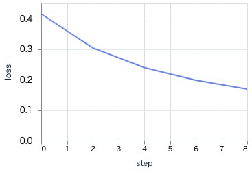
実行すると、エポック単位でグラフが更新され、学習が進むにつれ損失が下がり、正解率が上がっていることが分かります
最終的なグラフはそれぞれ以下のようになりました
-
損失
-
正解率
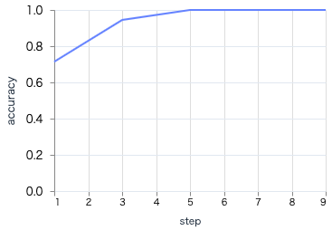
グラフの形状から、学習が問題なく進行したことが分かります
テストデータによる評価
テストデータに対して推論を実行し、正しく予測できているか確認します
まずは1件のデータだけで推論します
test_datum =
  %{
    "input1" => Nx.tensor([[0]]),
    "input2" => Nx.tensor([[0]])
  }
Axon.predict で推論を実行します
Axon.predict(model, trained_state, test_datum)
実行結果は以下のようになります
#Nx.Tensor<
  f32[1][1]
  EXLA.Backend<host:0, 0.2471620236.1584005131.198547>
  [
    [0.14083826541900635]
  ]
>
0.14083826541900635 は 1 よりも 0 に近く、入力の 0, 0 から OR 演算結果の 0 を正しく予測できました
では、すべての 0 1 の組み合わせで確認してみましょう
推論を実行する関数を用意します
predict = fn model, trained_state, {input_1, input_2} ->
  %{
    "input1" => Nx.tensor([[input_1]]),
    "input2" => Nx.tensor([[input_2]])
  }
  |> then(&Axon.predict(model, trained_state, &1))
  |> then(& &1[[0, 0]])
  |> Nx.to_number()
end
実行すると、先ほどと同じ 0.14083826541900635 が取得できました
predict.(model, trained_state, {0, 0})
入力としてすべての組み合わせを用意し、それぞれの実行結果をテーブル表示します
[
  {0, 0},
  {0, 1},
  {1, 0},
  {1, 1}
]
|> Enum.map(fn {input_1, input_2} ->
  predicted_value = predict.(model, trained_state, {input_1, input_2})
  predicted_label = if predicted_value < 0.5 do 0 else 1 end

  %{
    "input1" => input_1,
    "input2" => input_2,
    "value" => predicted_value,
    "label" => predicted_label
  }
end)
|> Kino.DataTable.new()
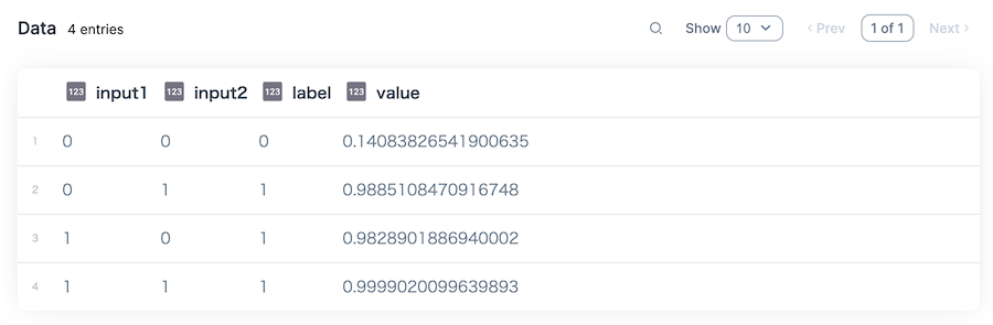
すべての結果が正しいですね
Elixirで機械学習に初挑戦③:「予測」の可視化と「精度」の変化要因、「学習過程グラフ」の読み方
モデルの内容や学習過程に関する解説がありました
推論の可視化
本来は論理演算なので 0 か 1 の不連続な値ですが、入力に小数値を与えてみましょう
plot = fn trained_state, model ->
  x =
    0..99
    |> Enum.map(&(&1 / 100))
    |> Nx.tensor()
    |> Nx.new_axis(1)

  y = Axon.predict(model, trained_state, %{"input1" => x, "input2" => x})

  points =
    [Nx.to_flat_list(x), Nx.to_flat_list(y)]
    |> Enum.zip()
    |> Enum.map(fn {x, y} -> %{x: x, y: y} end)

  VegaLite.new(width: 600, height: 400)
  |> VegaLite.data_from_values(points)
  |> VegaLite.mark(:line)
  |> VegaLite.encode_field(:x, "x", type: :quantitative)
  |> VegaLite.encode_field(:y, "y", type: :quantitative)
  |> Kino.VegaLite.new()
end
以下のような入力値に対して、それぞれの推論結果をプロットします
- 0.00, 0.00
- 0.01, 0.01
- 0.02, 0.02
... - 0.98, 0.98
- 0.99, 0.99
- 1.00, 1.00
plot.(trained_state, model)
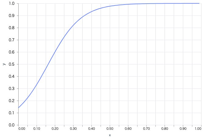
入力が 0,0 では予測は 0 に近く、そこを離れるとすぐに予測は 1 に近づいています
学習率の影響
学習率を引数として学習する関数を用意します
学習率による影響を分かりやすくするため、エポック数は1にします
fit = fn learning_rate, model ->
  model
  |> Axon.Loop.trainer(:binary_cross_entropy, Axon.Optimizers.sgd(learning_rate))
  |> Axon.Loop.metric(:accuracy, "accuracy")
  |> Axon.Loop.run(train_data, %{}, epochs: 1, iterations: 1000, compiler: EXLA)
end
学習率を 0.01 から 0.10 まで変化させてみます
1..10
|> Enum.map(& &1/100)
|> Enum.map(fn learning_rate ->
  {
    "lr=#{learning_rate}",
    learning_rate
    |> fit.(model)
    |> plot.(model)
  }
end)
|> Kino.Layout.tabs()
学習率が高いほど、より大きくパラメータを更新するため、1エポックだけでも学習が進んでいます(0, 0 のときの予測が 0 に近づき、より早い段階で予測が 1 に近づいている)
もちろん、実際には過学習の要因になるので大きければ大きいほど良いものではありません
まとめ
Livebook ではグラフ更新を簡単にアニメーション化できるため、楽に学習の推移を見守ることができます
もっといろんなモデルの学習を実行してみたいですね
次回はこちら