Elixir Livebook で農林水産省の筆ポリゴンデータを可視化する（田畑の形を地図上にプロットする）

はじめに

皆さん、お米食べてますか？

美味しいお米を生産してくれる田んぼは日本の宝です

というわけで、今回は農林水産省の筆（ふで）ポリゴンデータを使って、田んぼや畑を地図上にプロットしていきます

ちなみに、「筆」は登記するときの土地の単位です

例によって可視化には Elixir Livebook を使います

手軽に綺麗な可視化ができるからです

実装したノートブックはこちら

出典

「筆ポリゴンデータ（2022年度公開）」（農林水産省）（https://www.maff.go.jp/j/tokei/porigon/）を加工して作成

参考サイト

宙畑の Python 実装を参考にしています

「衛星データ利用環境整備・ソリューション開発支援事業」

この記事は経済産業省の「衛星データ利用環境整備・ソリューション開発支援事業」に関連して、衛星データを Elixir で処理する方法を研究するために書いています

近日、本記事で扱う地理情報と、 Tellus から取得する衛星データの紐付けについて記事を投稿します

実行環境

• macOS Ventura 13.1
• Rancher Desktop 1.7.0

Livebook 0.8.0 の Docker　イメージを元にしたコンテナで動かしました

コンテナ定義はこちらを参照

セットアップ

Livebook のセットアップセル（先頭のセル）に以下を入力して実行します

Mix.install(
  [
    {:nx, "~> 0.4"},
    {:evision, "~> 0.1"},
    {:exla, "~> 0.4"},
    {:geo, "~> 3.4"},
    {:jason, "~> 1.4"},
    {:kino, "~> 0.8"},
    {:kino_maplibre, "~> 0.1.3"}
  ],
  config: [
    nx: [
      default_backend: EXLA.Backend
    ]
  ]
)

以下の依存モジュールをインストールしています

• Nx: 行列演算
• Evision: 画像処理
• EXLA: 行列演算の高速化
• Geo: 地理情報システム
• Jason: JSONパーサー
• Kino: Livebook での入出力
• Kino MapLibre: 地図出力

また、 Nx による行列演算を EXLA を使って高速化する設定をしています

筆ポリゴンデータのダウンロード

筆ポリゴン公開サイトから画面下部の「筆ポリゴンデータダウンロードページ」のボタンをクリックします

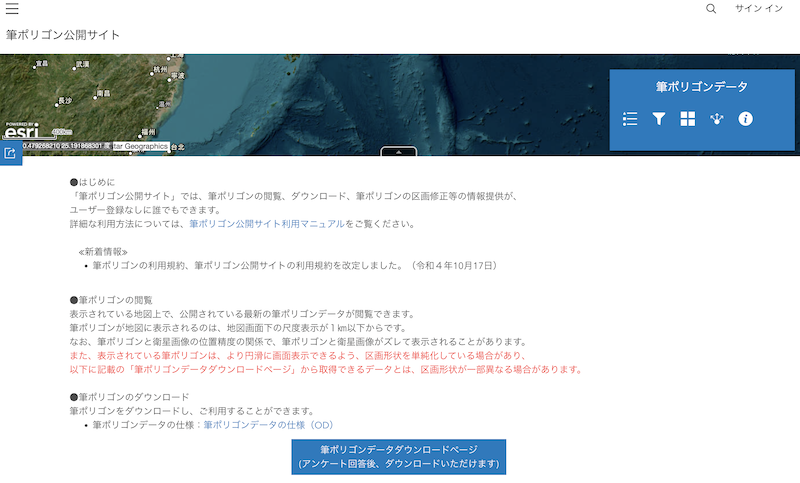
表示されるアンケートに回答します

遷移先のダウンロードページで公開年度、都道府県、市区町村を選択し、「ダウンロード」をクリックします

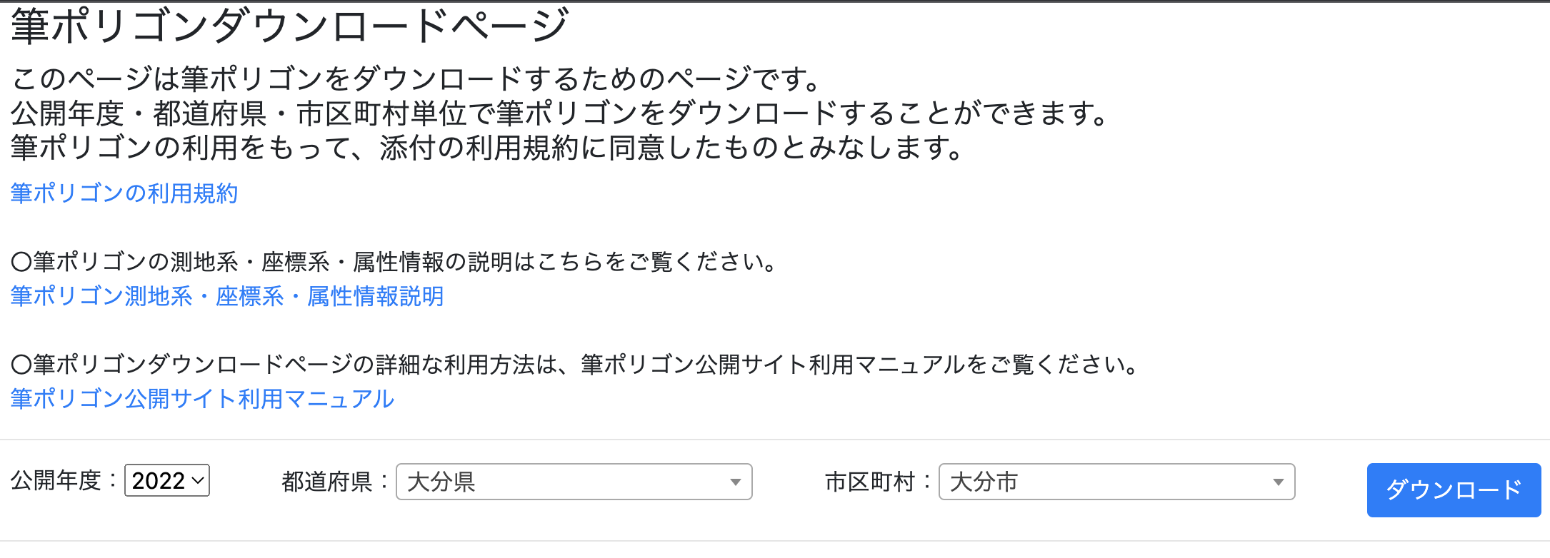
ダウンロードした ZIP ファイルを展開します

今回は大分県大分市 2022 年度のデータを /tmp/2022_442011.json に展開したものとして進めます

拡張子は単に .json ですが、中身は　GeoJSON になっています

GeoJSON は地理情報を JSON 形式で表現するための形式です

Elixir では Geo モジュールを使うことで扱いやすくすることができます

GeoJSON の読込

json ファイルを開いて見ましょう

geojson_data =
  json_file
  |> File.read!()
  |> Jason.decode!()
  |> Geo.JSON.decode!()

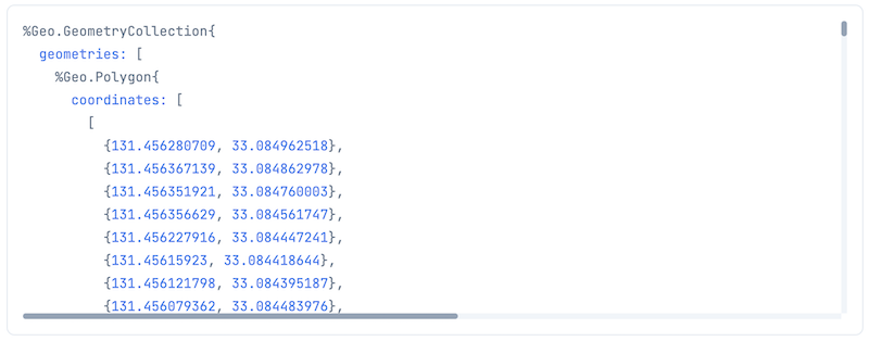
パースした結果は以下のような形式になっています

データの仕様はこちら

%Geo.GeometryCollection{
  geometries: [
    # 田畑の地理情報
    %Geo.Polygon{
      coordinates: [
        # 一つのポリゴン
        [
          [
            {<経度>, <緯度>},
            {<経度>, <緯度>},
            {<経度>, <緯度>},
            ...
          ]
        ]
      ],
      srid: nil,
      properties: %{
        "edit_year" => <調製年度>,
        "history" => <履歴>,
        "issue_year" => <公開年度>,
        "land_type" => <耕地の種類:地目コード（100：田、200：畑）>,
        "last_polygon_uuid" => <前年筆ポリゴンID>,
        "local_government_cd" => <地方公共団体コード>,
        "point_lat" => <重心点座標緯度>,
        "point_lng" => <重心点座標経度>,
        "polygon_uuid" => <筆ポリゴンID>,
        "prev_last_polygon_uuid" => <前前年筆ポリゴンID>
      }
    },
    %Geo.Polygon{
      ...

地理情報は、このように緯度と経度で表される地球上の点を複数列挙し、その点を結ぶ多角形（ポリゴン）で表現されます

Enum.count(geojson_data.geometries)

件数をカウントしてみます

64,400 件ありました

田んぼだけだと 37,817 件

geojson_data.geometries
|> Enum.filter(& &1.properties["land_type"] == 100)
|> Enum.count()

畑だけだと 26,583 件

# 畑の件数
geojson_data.geometries
|> Enum.filter(& &1.properties["land_type"] == 200)
|> Enum.count()

件数が大きすぎるため、緯度経度で絞り込みます

target_fields =
  geojson_data.geometries
  |> Enum.filter(fn field ->
    field.properties["point_lng"] >= 131.42 &&
    field.properties["point_lng"] <= 131.46 &&
    field.properties["point_lat"] >= 33.13 &&
    field.properties["point_lat"] <= 33.15 &&
    field.properties["land_type"] == 100
  end)
  |> then(fn geometries ->
    %Geo.GeometryCollection{geometries: geometries}
  end)

Enum.count(target_fields.geometries)

Smart Cell による可視化

Livebook ではこの GeoJSON データを Smart Cell に渡すだけで簡単に可視化できます

セルを追加するときに +Smart を開き、 Map を選択します

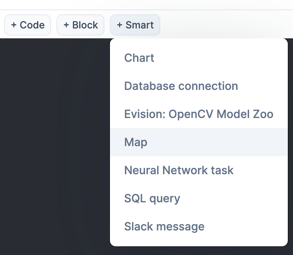
追加された　Smart Cell　に値を指定します

• MAP STYLE: terrain(non-commercial)
• CENTER: 131.443, 33.131
• ZOOM: 16
• Source: target_fields
• Type: line

セルを実行すると、航空写真の地図上に田んぼの形が表示されます

この地図はズームしたり表示範囲を動かしたり、対話的（インタラクティブ）に動作します

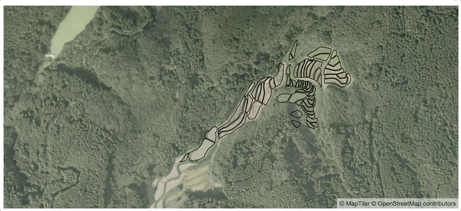
この黒い線の折れている点全ての座標が GeoJSON の中に書かれているわけです

Smart Cell を使わない可視化

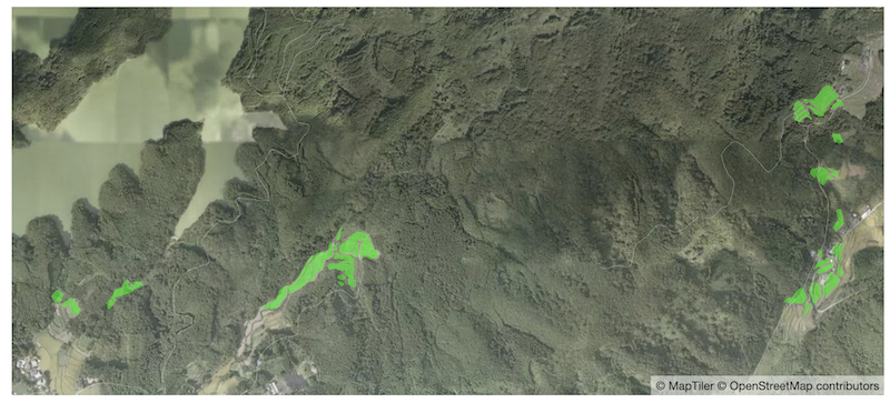
Smart Cell を使わず、最初から当該区域を中心にズームして、田んぼを塗りつぶしてみましょう

中心座標を取得します

longitudes =
  target_fields.geometries
  |> Enum.map(& &1.coordinates)
  |> List.flatten()
  |> Enum.map(&elem(&1, 0))

latitudes =
  target_fields.geometries
  |> Enum.map(& &1.coordinates)
  |> List.flatten()
  |> Enum.map(&elem(&1, 1))

center = {
  (Enum.min(longitudes) + Enum.max(longitudes)) / 2,
  (Enum.min(latitudes) + Enum.max(latitudes)) / 2
}

MapLibre に GeoJSON を渡してプロパティを指定し、可視化します

MapLibre.new(center: center, zoom: 14.5, style: :terrain)
|> MapLibre.add_geo_source("geojson", target_fields)
|> MapLibre.add_layer(
  id: "fill",
  source: "geojson",
  type: :fill,
  # 半透明の緑にする
  paint: [fill_color: "#00ff00", fill_opacity: 0.5]
)

Evision による可視化

では Evision を使って、この多角形を画像データにしてみましょう

まず、対象区域の端の緯度経度を取得します

# 緯度経度の最大最小を求める
coordinates =
  target_fields.geometries
  |> Enum.map(& &1.coordinates)
  |> List.flatten()

longitudes = Enum.map(coordinates, &elem(&1, 0))
latitudes = Enum.map(coordinates, &elem(&1, 1))

min_longitude = Enum.min(longitudes)
max_longitude = Enum.max(longitudes)
min_latitude = Enum.min(latitudes)
max_latitude = Enum.max(latitudes)

{min_longitude, max_longitude, min_latitude, max_latitude}

画像にするときのサイズを指定します

{height, width} = {1280, 2560}

緯度経度の最小から最大をピクセル数の0から幅・高さに正規化します

大分県の場合は以下のようになります

• 横方向:
  • 正規化前: 131.435353795 から 131.460065396
  • 正規化後: 0 から 1280
• 縦方向:
  • 正規化前: 33.135901549 から 33.129839302
  • 正規化後: 0 から 2560

縦方向は北緯なので大小が逆転します

normalized_points =
  target_fields.geometries
  |> Enum.map(& &1.coordinates)
  |> Enum.map(fn coordinate ->
    coordinate
    |> Enum.at(0)
    |> Enum.map(fn {x, y} ->
      [
        trunc((x - min_longitude) * width / (max_longitude - min_longitude)),
        # 縦方向は緯度が北緯の場合逆転するため、高さから引く
        trunc(height - (y - min_latitude) * height / (max_latitude - min_latitude))
      ]
    end)
    |> Nx.tensor(type: :s32)
  end)

多角形を描画するための空画像を用意します

透明度を使うため、 BGRA の4つに 0 を指定します

# 全て黒の不透明
empty_mat =
  [0, 0, 0, 255]
  |> Nx.tensor(type: :u8)
  |> Nx.tile([height, width, 1])
  |> Evision.Mat.from_nx_2d()

Evision.fillPoly に元画像、多角形の配列、色を渡すことで画像に多角形を描画できます

img = Evision.fillPoly(empty_mat, normalized_points, {0, 0, 0, 0})

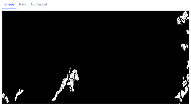
縦 1280 ピクセル、横 2560 ピクセルに田んぼの形を多角形として表現できました

白いところは透明になっています

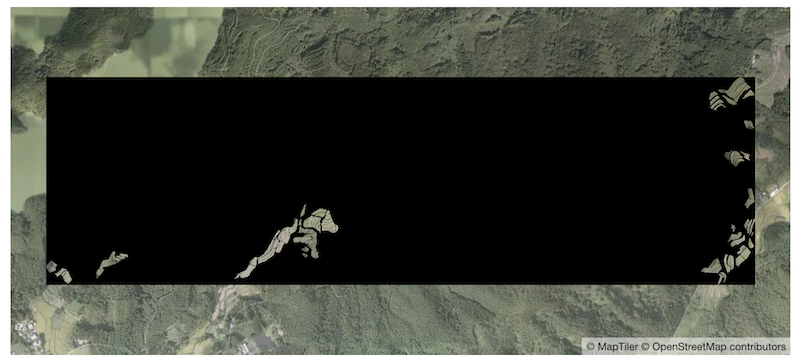
これを地図上にプロットしてみます

画像を地図にプロットするため、 BASE64 にします

img_base64 =
  Evision.imencode(".png", img)
  |> Base.encode64()
  |> then(&"data:image/png;base64,#{&1}")

MapLibre.new(center: center, zoom: 14.5, style: :terrain)
# 画像をレイヤーとして地図に重ねる
|> MapLibre.add_source(
  "field_mask",
  type: :image,
  url: img_base64,
  coordinates: [
    [min_longitude, max_latitude],
    [max_longitude, max_latitude],
    [max_longitude, min_latitude],
    [min_longitude, min_latitude]
  ]
)
|> MapLibre.add_layer(
  id: "overlay",
  source: "field_mask",
  type: :raster,
  layout: %{
    "visibility" => "visible"
  }
)

まとめ

画像データ化できた筆ポリゴンデータに衛星データから計算した植生（どれくらい植物が生えているか）を重ねることで、田畑の栽培状況を見ることができます

別のオープンデータを使えば都道府県や市区町村も地図上にプロットできます