Additional Content

Geometric Weighting Implementation
By executing the code below, we can know that the geometric weights sum to 1.
def f(a,n):
	b = 0
	for i in range(n):
		b += (1 - a)*(a**(i))
	return b

print(f(0.01, 2))
# 0.999
Mathematical Proof
\sum ^{n}_{i=0} r^i = \frac{1-r^{n+1}}{1-r}\\
Hence\\
(1 - r)\sum ^{n}_{i=0} r^i = 1-r^{n+1}
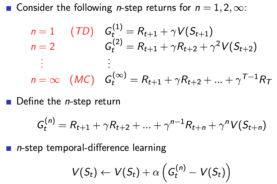
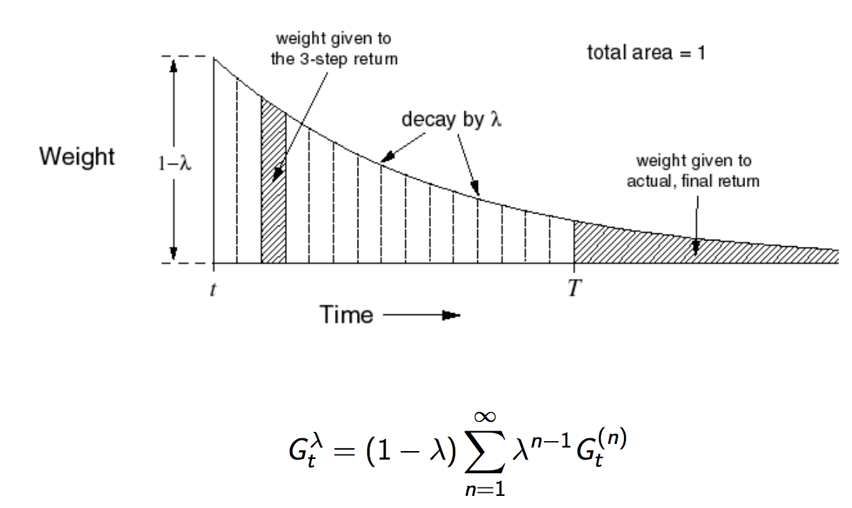
Forward View TD(λ)
 1. Like MC, FTD can only look forward and never learn from incomplete episodes.
2. Updates the value functions towards $\lambda$ returns.
1. Like MC, FTD can only look forward and never learn from incomplete episodes.
2. Updates the value functions towards $\lambda$ returns.
G^{\lambda}_t = (1 - \lambda) \sum^{\infty}_{n-1}\lambda^{n-1}G^n_t
Eligibility Traces (Credit Assignment Problem)
Which step does affect most the consequence?? => there are two major ways to evaluate the importance of steps.
- Frequency heuristic : assign credit to most frequent states
- Recency heuristic : assign credit to most recent states
ET combines them.
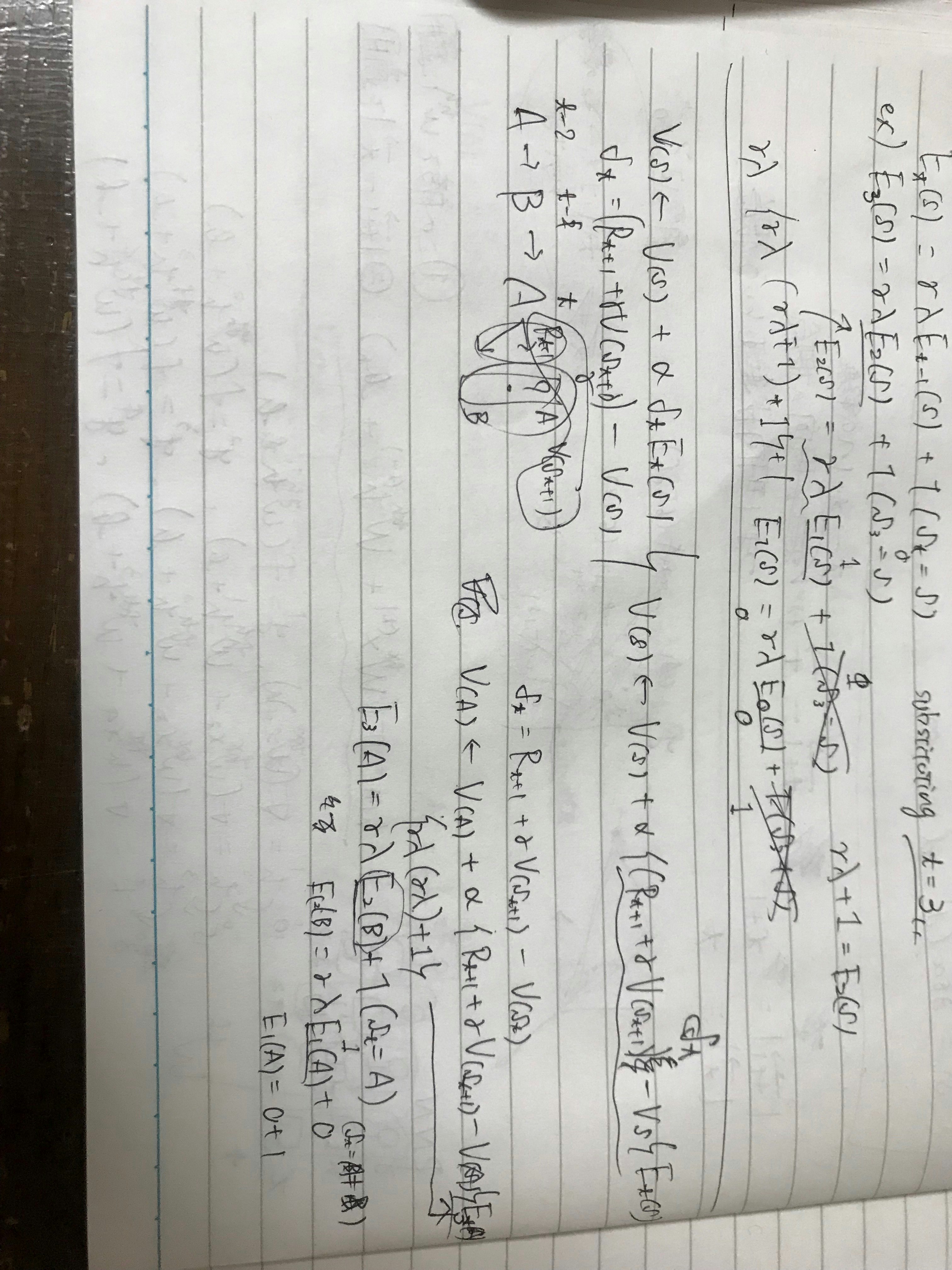
E_0(s) = 0\\
E_t(s) = γλE_{t−1}(s) + 1(S_t = s)
ex1) Let t be 3, and $S_3 = s_3 = s_2 = s_1$
*This means, we simple consider loopy situation, like A -> A -> A.
E_3(s_3) = γλE_{2}(s_3) + 1(S_3 = s_3)\\
E_2(s) = γλE_{1}(s) + 1(S_3 = s_2)\\
E_1(s) = γλE_{0}(s) + 1(S_3 = s_1)\\
E_0(s) = 0\\
Hence\\
E_3(s) = γλ \space \bigl(\space γλ \space(\space γλ + 1 \space )_1 + 1 \space \bigl)_2 \space +1
ex2) Let t be 3, and $S_3 = s_3 = s_1 \neq s_2$
*This means, we simple consider loopy situation, like A -> B -> A.
E_3(s_3) = γλE_{2}(s_3) + 1(S_3 = s_3)\\
E_2(s) = γλE_{1}(s) + 0(S_3 \neq s_2)\\
E_1(s) = γλE_{0}(s) + 1(S_3 = s_1)\\
E_0(s) = 0\\
Hence\\
E_3(s) = γλ \space \bigl(\space γλ \space(\space γλ + 1 \space )_1 \space \bigl)_2 \space +1
So if the state frequently happens, then from the perspective of both frequency and recency, the importance of that state increases, vice versa.
We are going to apply this technique in BTD algo below.
Backward View TD(λ)

- Keep an eligibility trace for every state s
- Update value V(s) for every state s
- In proportion to TD-error δt and eligibility trace Et(s)
δ_t = R_{t+1} + γV(S_{t+1}) − V(S_t)\\
V(s) ← V(s) + αδ_tE_t(s)\\
Ex1) Let λ be 0, This is exactly equivalent to TD(0) update
E_t(s) = 1(S_t = s)\\
V(s) ← V(s) + αδ_tE_t(s) \equiv V(S_t) ← V(S_t) + αδ_t\\
Ex2)
Check the part below the line.
All in all, we have seen two methods for updating Temporal Difference, Forward and Backward view.
Technically speaking, both methods explicitly incorporate the time handling approach, which is calculation of $G^λ_t$ and Eligibility Traces respectively.
$G^λ_t$: look the future till the terminal state
Eligibility Traces: look back till the beginning
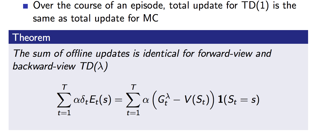
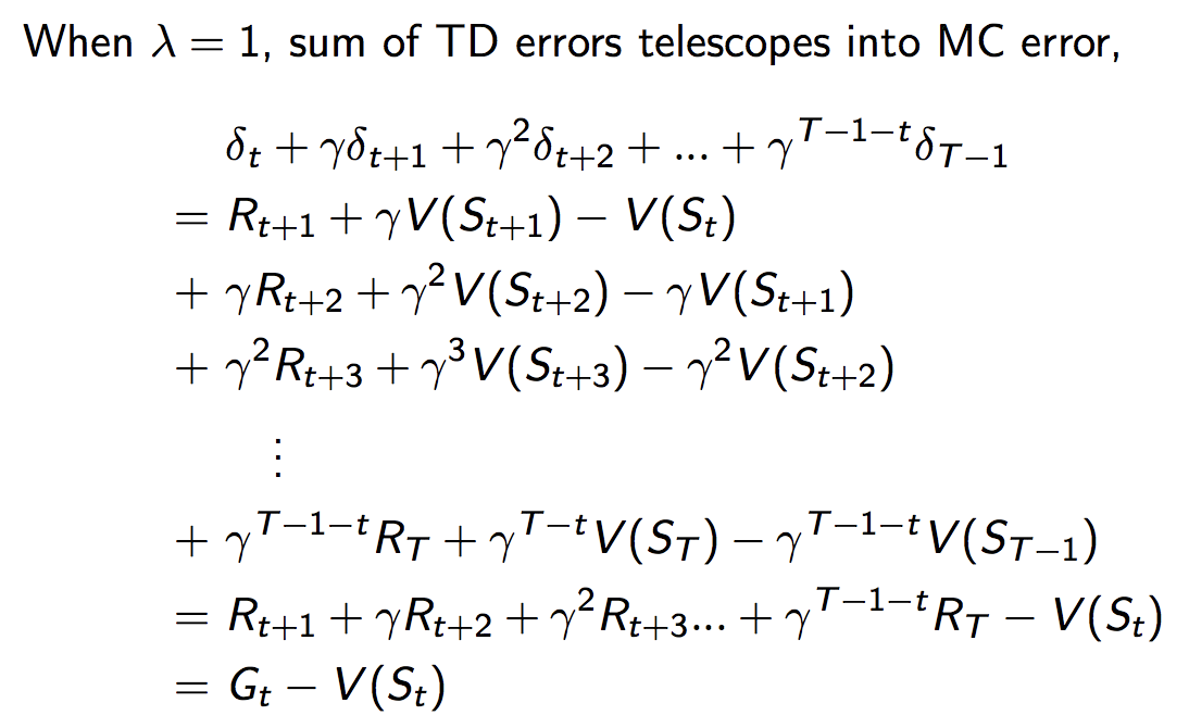
Equivalence of TD(λ) and MC
Over the course of an episode, total update for TD(1) is the same as total update for MC.
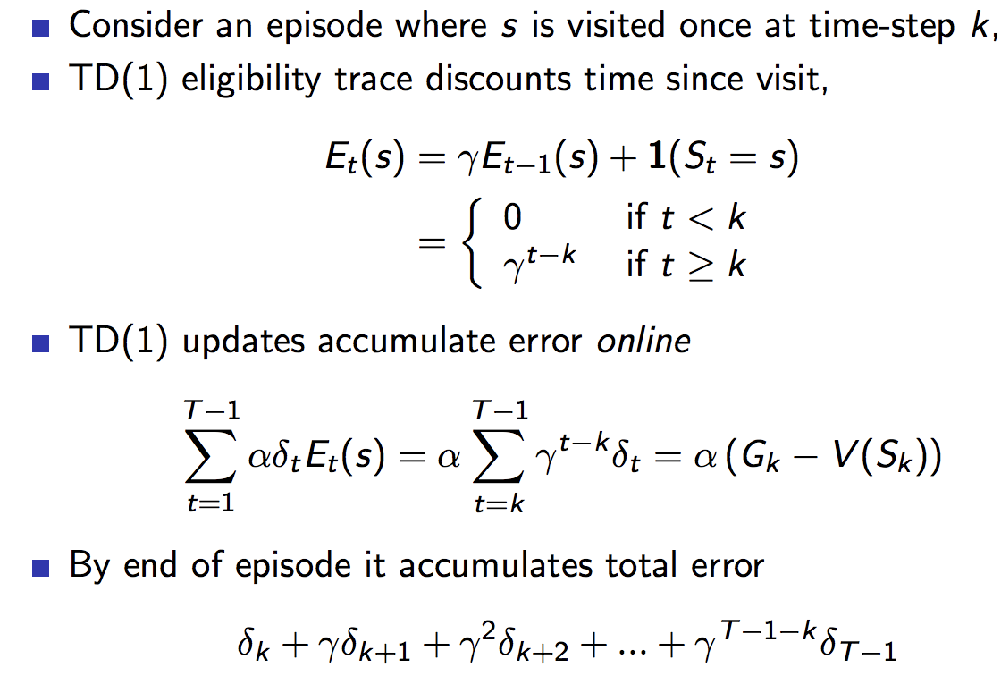
Manual Explanation
Case λ be 1.
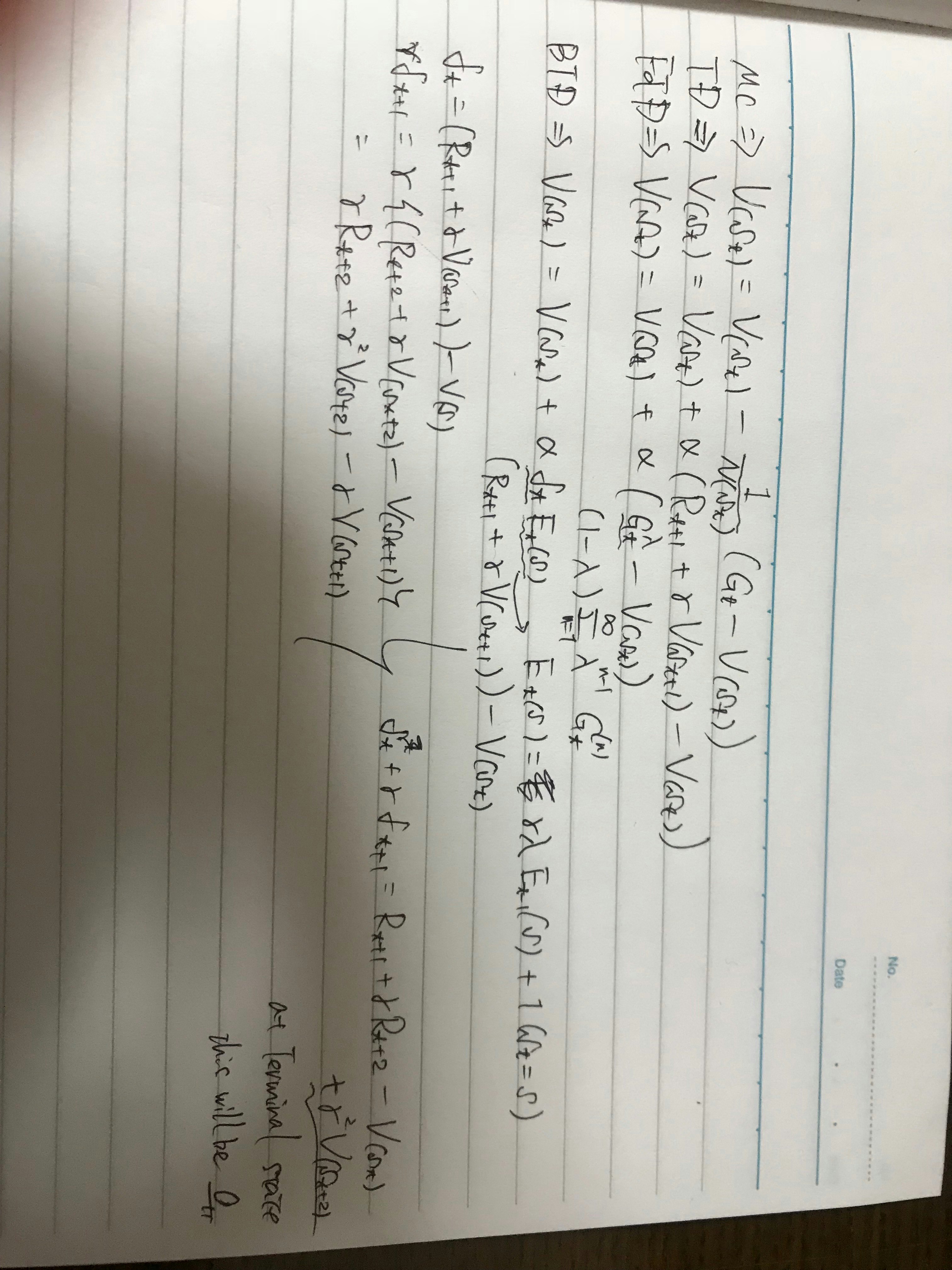
So, the intermediate $\gamma V(S_{t+1})$ will be offset by TD error of next step.
Bear in mind that at the terminal step, $V(S)$ becomes 0.