はじめに: 問題設定
10クラスの画像を分類する、画像ベースの分類問題をときます。
データセット概論
一般的に、画像、テキスト、音声、動画などのデータを扱う場合は、numpy配列にデータを読み込むことや、標準的なPythonパッケージを利用することができます。そして、numpy配列からtorch.*Tensorを用いて、テンソルに変換することが可能です。
- 画像の場合は、Pillow、OpenCVなどのパッケージが便利です
- 音声に対しては scipy や librosa などのパッケージがあります
- テキストの場合は、そのままのPythonまたはCythonによる読み込み、もしくはNLTKやSpaCyが便利です
今回のデータセット
「CIFAR10データセット」を使用します。
このデータセットには「飛行機」、「自動車」、「鳥」、「猫」、「鹿」、「犬」、「カエル」、「馬」、「船」、「トラック」のクラスが含まれています。
また、CIFAR-10の画像はサイズが3×32×32、すなわち3つの色チャネルを持つ32×32ピクセルの画像になります。
画像分類器の訓練
以下の手順に従って実施します:
- torchvisionを用いた、CIFAR10の訓練データとテストデータの読み込みと正規化
- 畳み込みニューラルネットワークの定義
- 損失関数の定義
- 訓練データを用いたネットワークの訓練
- テストデータでネットワークをテスト
CIFAR10の読み込みと正規化
libraryを読み込む
import torch
import torchvision
import torch.optim as optim
import torch.nn as nn
import torch.nn.functional as F
import torchvision.transforms as transforms

import random
import numpy as np
import matplotlib.pyplot as plt

# random seedを設定
seed = 2023
torch.manual_seed(seed)
torch.cuda.manual_seed_all(seed)
np.random.seed(seed)
random.seed(seed)
torch.backends.cudnn.benchmark = False
torch.backends.cudnn.deterministic = True
torchvisionデータセットの出力は、値が0から1の範囲のPILImageイメージになります。
これを値が-1から1の範囲に付近に正規化されたTensor(テンソル)に変換します。
transform = transforms.Compose(
    [transforms.ToTensor(),
     transforms.Normalize((0.5, 0.5, 0.5), (0.5, 0.5, 0.5))])

trainset = torchvision.datasets.CIFAR10(root='./data', train=True,
                                        download=True, transform=transform)
trainloader = torch.utils.data.DataLoader(trainset, batch_size=4,
                                          shuffle=True, num_workers=2)

testset = torchvision.datasets.CIFAR10(root='./data', train=False,
                                       download=True, transform=transform)
testloader = torch.utils.data.DataLoader(testset, batch_size=4,
                                         shuffle=False, num_workers=2)

classes = ('plane', 'car', 'bird', 'cat',
           'deer', 'dog', 'frog', 'horse', 'ship', 'truck')
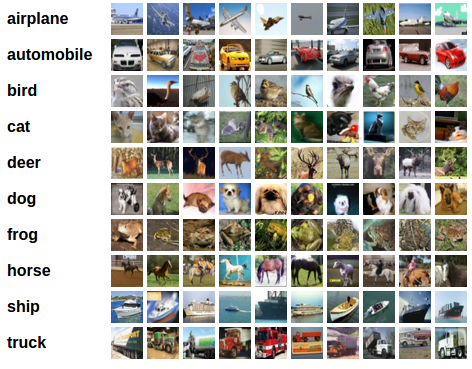
それでは訓練画像を楽しく眺めてみましょう。
def imshow(img):  # 画像の表示関数
    img = img / 2 + 0.5     # 正規化を戻す
    npimg = img.numpy()
    plt.imshow(np.transpose(npimg, (1, 2, 0)))
    plt.show()


# 適当な訓練セットの画像を取得
dataiter = iter(trainloader)
images, labels = next(dataiter)

# 画像の表示
imshow(torchvision.utils.make_grid(images))
# ラベルの表示
print(' '.join('%5s' % classes[labels[j]] for j in range(4)))

畳み込みニューラルネットワークの定義
CNNを定義し、3chのカラー画像を入力にとる
class Net(nn.Module):
    def __init__(self):
        super(Net, self).__init__()
        self.conv1 = nn.Conv2d(3, 6, 5)
        self.pool = nn.MaxPool2d(2, 2)
        self.conv2 = nn.Conv2d(6, 16, 5)
        self.fc1 = nn.Linear(16 * 5 * 5, 120)
        self.fc2 = nn.Linear(120, 84)
        self.fc3 = nn.Linear(84, 10)

    def forward(self, x):
        x = self.pool(F.relu(self.conv1(x)))
        x = self.pool(F.relu(self.conv2(x)))
        x = x.view(-1, 16 * 5 * 5)
        x = F.relu(self.fc1(x))
        x = F.relu(self.fc2(x))
        x = self.fc3(x)
        return x

device = "cuda"
net = Net().to(device)
学習部分の定義
再利用しやすいように、関数で定義する
def train(net, opt, criterion, num_epochs=10):
    """
    データの繰り返し処理を実行し、入力データをネットワークに与えて最適化します
    """
    # 学習経過を格納するdict
    history = {"loss":[], "accuracy":[], "val_loss":[], "val_accuracy":[]}

    for epoch in range(num_epochs):
        train_loss = 0.
        train_acc = 0.
        valid_loss = 0.
        valid_acc = 0.
        train_total = 0
        valid_total = 0

        # 学習
        for data in trainloader:
            inputs, labels = data[0].to(device), data[1].to(device)
            opt.zero_grad() # 勾配情報をリセット
            pred = net(inputs)  # モデルから予測を計算(順伝播計算):tensor(BATCH_SIZE, 確率×10)
            loss = criterion(pred, labels) # 誤差逆伝播の微分計算
            train_loss += loss.item() # 誤差(train)を格納
            loss.backward()
            opt.step()  # 勾配を計算
            _, indices = torch.max(pred.data, axis=1)  # 最も確率が高いラベルの確率と引数をbatch_sizeの数だけ取り出す
            train_acc += (indices==labels).sum().item() # labelsと一致した個数
            train_total += labels.size(0) # データ数(=batch_size)

        history["loss"].append(train_loss)  # 1epochあたりの誤差の平均を格納
        history["accuracy"].append(train_acc/train_total) # 正解数/使ったtrainデータの数

        # 学習ごとの検証
        with torch.no_grad():
            for data in testloader:
                inputs, labels = data[0].to(device), data[1].to(device)
                pred = net(inputs)  # モデルから予測を計算(順伝播計算):tensor(BATCH_SIZE, num_class)
                loss = criterion(pred, labels) # 誤差の計算
                valid_loss += loss.item()  # 誤差(valid)を格納
                values, indices = torch.max(pred.data, axis=1)  # 最も確率が高い引数をbatch_sizeの数だけ取り出す
                valid_acc += (indices==labels).sum().item()
                valid_total += labels.size(0) # データ数(=batch_size)

        history["val_loss"].append(valid_loss)  # 1epochあたりの検証誤差の平均を格納
        history["val_accuracy"].append(valid_acc/valid_total) # 正解数/使ったtestデータの数
        # 5の倍数回で結果表示
        if (epoch+1)%5==0:
            print(f'Epoch:{epoch+1:d} | loss:{history["loss"][-1]:.3f} accuracy: {history["accuracy"][-1]:.3f} val_loss: {history["val_loss"][-1]:.3f} val_accuracy: {history["val_accuracy"][-1]:.3f}')
    return net, history
トレーニング
criterion = nn.CrossEntropyLoss()
# opt = optim.SGD(net.parameters(), lr=0.001, momentum=0.9)
opt = optim.Adam(net.parameters(), lr=0.001)
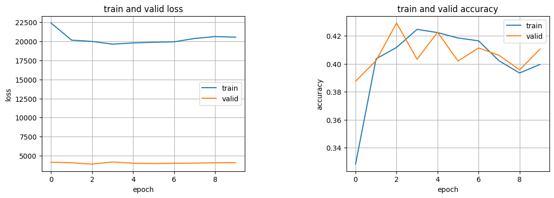
net, history = train(net=net, opt=opt, criterion=criterion)
学習経過の描画
plot_figでは、学習の経過を描画している。
** ここはkerasの時とほぼ同じで、historyの中身をmatplotlibを使って描画している。
def plot_fig(history):
    plt.figure(1, figsize=(13,4))
    plt.subplots_adjust(wspace=0.5)

    # 学習曲線
    plt.subplot(1, 2, 1)
    plt.plot(history["loss"], label="train")
    plt.plot(history["val_loss"], label="valid")
    plt.title("train and valid loss")
    plt.xlabel("epoch")
    plt.ylabel("loss")
    plt.legend()
    plt.grid()

    # 精度表示
    plt.subplot(1, 2, 2)
    plt.plot(history["accuracy"], label="train")
    plt.plot(history["val_accuracy"], label="valid")
    plt.title("train and valid accuracy")
    plt.xlabel("epoch")
    plt.ylabel("accuracy")
    plt.legend()
    plt.grid()

    plt.show()

plot_fig(history=history)
テストデータでネットワークをテスト
ネットワークがきちんと学習したかどうかを確かめる必要があります。ニューラルネットワークの出力である画像のカテゴリラベルを予測し、正解ラベルと比較します。予測結果が正しければ、そのサンプルを正しい予測結果リストに追加します。
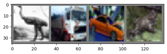
まずはテストセットに慣れるために、テスト画像を表示。
dataiter = iter(testloader)
inputs, labels = next(dataiter)
inputs, labels = inputs.to(device), labels.to(device)

# 画像と正解ラベルの表示
imshow(torchvision.utils.make_grid(images))
print('GroundTruth: ', ' '.join('%5s' % classes[labels[j]] for j in range(4)))
そして、ニューラルネットワークが上記の入力を、どのように捉えたのか確認しましょう。出力は入力画像に対する10個のカテゴリの"エネルギー"(のようなもの)を表しています。とあるカテゴリのエネルギーが高いほど、ネットワークはその画像がそのカテゴリに属すると考えます。ですので、エネルギーが最も高いカテゴリを取得しましょう:
outputs = net(inputs)
_, predicted = torch.max(outputs, 1)

print('Predicted: ', ' '.join('%5s' % classes[predicted[j]] for j in range(4)))

"""
>> Predicted:    cat  ship plane plane
"""
ネットワークがデータセット全体に対しどの程度の性能になっているか確認しましょう。
correct = 0
total = 0
with torch.no_grad():
    for data in testloader:
        inputs, labels = data[0].to(device), data[1].to(device)
        outputs = net(inputs)
        _, predicted = torch.max(outputs.data, 1)
        total += labels.size(0)
        correct += (predicted == labels).sum().item()

print('Accuracy of the network on the 10000 test images: %d %%' % (100 * correct / total))

"""
>> Accuracy of the network on the 10000 test images: 60 %
"""
ネットワークが何らかを学習しているようです。 ではうまく分類できたクラス、できなかったクラスはそれぞれ何だったのでしょうか:
class_correct = list(0. for i in range(10))
class_total = list(0. for i in range(10))
with torch.no_grad():
    for data in testloader:
        inputs, labels = data[0].to(device), data[1].to(device)
        outputs = net(inputs)
        _, predicted = torch.max(outputs, 1)
        c = (predicted == labels).squeeze()
        for i in range(4):
            label = labels[i]
            class_correct[label] += c[i].item()
            class_total[label] += 1

for i in range(10):
    print('Accuracy of %5s : %2d %%' % (classes[i], 100 * class_correct[i] / class_total[i]))

"""
>>
Accuracy of plane : 65 %
Accuracy of   car : 76 %
Accuracy of  bird : 50 %
Accuracy of   cat : 32 %
Accuracy of  deer : 52 %
Accuracy of   dog : 48 %
Accuracy of  frog : 74 %
Accuracy of horse : 65 %
Accuracy of  ship : 71 %
Accuracy of truck : 72 %
"""
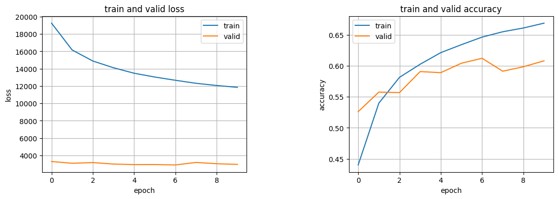
次にもう少し層の深いネットワークを試してみる
class CNN(nn.Module):
  def __init__(self, num_class):
      super().__init__()
      self.feature = nn.Sequential(
          # ブロック1
          # (チャンネル数, フィルタ枚数, カーネルサイズ)
          nn.Conv2d(3, 128, kernel_size=3, padding=(1,1), padding_mode="replicate"),
          nn.ReLU(),
          nn.Conv2d(128, 128, kernel_size=3, padding=(1,1), padding_mode="replicate"),
          nn.ReLU(),
          nn.MaxPool2d((2,2)),
          nn.Dropout(0.25),

          # ブロック2
          nn.Conv2d(128, 64, kernel_size=3, padding=(1,1), padding_mode="replicate"),
          nn.ReLU(),
          nn.Conv2d(64, 64, kernel_size=3, padding=(1,1), padding_mode="replicate"),
          nn.ReLU(),
          nn.MaxPool2d((2,2)),
          nn.Dropout(0.25),

          # ブロック3
          nn.Conv2d(64, 32, kernel_size=3, padding=(1,1), padding_mode="replicate"),
          nn.ReLU(),
          nn.Conv2d(32, 32, kernel_size=3, padding=(1,1), padding_mode="replicate"),
          nn.ReLU(),
          nn.MaxPool2d((2,2)),
          nn.Dropout(0.25)
      )

      # 平滑化
      self.flatten = nn.Flatten()

      # 全結合
      self.classifier = nn.Sequential(
          nn.Linear(4*4*32, 512),
          nn.Dropout(0.6),
          nn.Linear(512, num_class)
      )

  def forward(self, input_data):
    input_data = self.feature(input_data)
    input_data = self.flatten(input_data)
    input_data = self.classifier(input_data)

    return input_data

net = CNN(num_class=10).to(device)

# トレーニング
criterion = nn.CrossEntropyLoss()
# opt = optim.SGD(net.parameters(), lr=0.001, momentum=0.9)
opt = optim.Adam(net.parameters(), lr=0.001)
net, history = train(net=net, opt=opt, criterion=criterion)
plot_fig(history=history)
hmmm,,, 悪くなってしまった。一概にdeepなモデルがいいわけではないのかもしれない。。