パーセプトロンについて

今回はパーセプトロンについてまとめたいと思います。

イントロ

機械学習を大別すると分類問題と数値問題に分けられます.
人間の脳細胞ニューロンをまね, コンピューター上で最初に表したものがパーセプトロン(perceptron)です.
1957年にローゼンブラット(Rosenblatt)によって,データを２つのクラスに線形で分離するために考案されたアルゴリズムです.
それゆえ非線形問題は解決できず, そのために多層パーセプトロンという、パーセプトロンを多層に重ねたアルゴリズムが考案されました.

ニューロンのイメージ

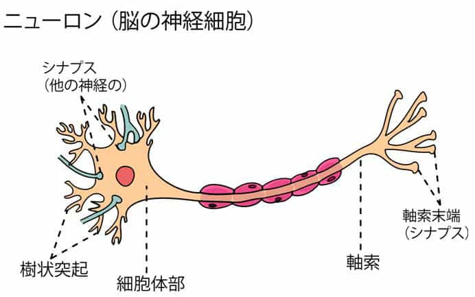
画像もと：http://tsushan.hatenadiary.jp/entry/2018/03/10/200305

数学的な背景

ここからちょっと数学的な背景の説明を行なっていきたいと思います。
まずはざっと数学的な記号を付した下記の図をご覧ください。

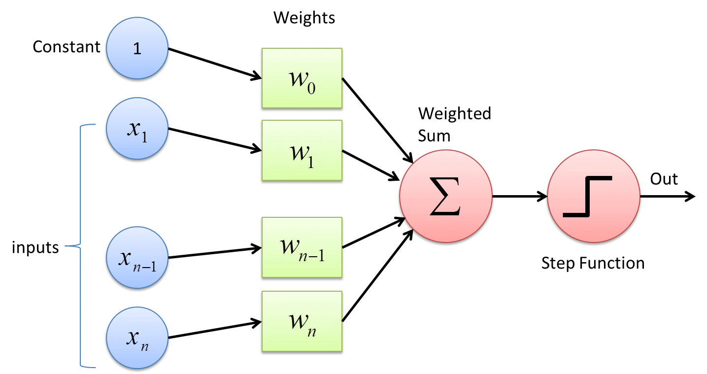
画像もと：https://towardsdatascience.com/what-the-hell-is-perceptron-626217814f53

そして、この図を元にパーセプトロンを数式で表すと次のように書けます.
また、数式内部の変数については、下記の様な読み替えをして見てください。

• $x$:入力
• $h_w(x)$:出力
• $w$:重み
• $b$:バイアス

\begin{align}
h_w (x) & = w_0＋w_1x_1+\cdots +w_nx_n\\
&= \sum_{i=0}^n w_ix_i\\
&=\boldsymbol{w}^T\boldsymbol{x}\\
\end{align}

ここまでの段階では、ただの線形回帰の式となんら変わりはございません。
しかし、パーセプトロンの違うところはここからになります。
このアルゴリズムを用いて線形分離をしていきたいので、この吐き出された $h_w (x) = \boldsymbol{w}^T\boldsymbol{x}$ に対して、閾値($\theta$)を設けます。

h_w (x) = \boldsymbol{w}^T\boldsymbol{x}  \geq \theta \\
or\\
h_w (x) = \boldsymbol{w}^T\boldsymbol{x}  < \theta \\

というにこの分け方ができます。
しかし、これでは見辛いので少々整形します。

h_w (x) = \left\{
\begin{array}{ll}
1 & (\boldsymbol{w}^T\boldsymbol{x} \geq \theta) \\
0 & (\boldsymbol{w}^T\boldsymbol{x} \lt \theta)
\end{array}
\right.

となります。
こちらを図示すると下記の様なグラフを描けます。

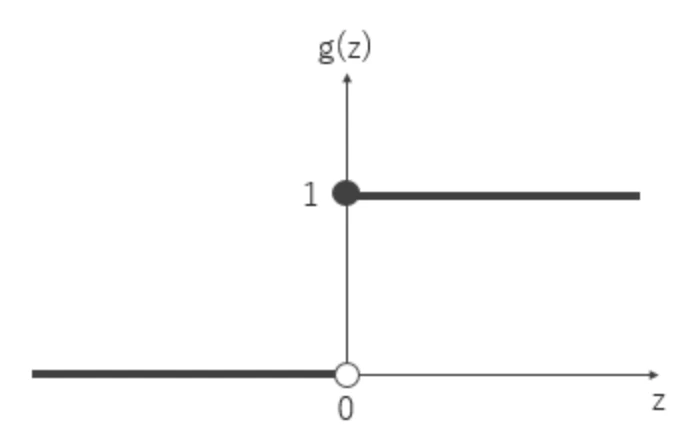
これが一般的にいう、ステップ関数というものになります。
基本的には線型性はなく、$x=0$の時点で、突如値が0から1へと飛び跳ねます。

• この図で言う、$g(z)$ は $h_w (x)$ と読み替えてください！

学習のアルゴリズム

学習アルゴリズムは次のステップで表すことができます.

1. 重み$w$を0か小さな乱数で初期化する
2. それぞれのトレーニングサンプルに対し
   1. 出力値$\hat{y}$を計算する
   2. 重み$w$を更新する

重みの更新の各iteration $\tau$は次のように書ける.

\begin{align}
\qquad & w_j^{\tau +1}=w_j^\tau +\Delta w_j^{\tau}\\
\Leftrightarrow &\quad w_j:=w_j+\Delta w_j\tag{5}
\end{align}

ここで$\Delta w$は正解の分類$y$, 予測された分類結果$\hat{y}$, 学習率 $\eta , (0\leq \eta \leq 1$)を用いて,

\Delta w_j=\eta (y^i - \hat{y}^i)x_j^i\tag{6}

また, このアルゴリズムは実質重みがかかる層は１層であるため (図1), 単層(単純)パーセプトロンとも呼ぶ.

アルゴリズムの最適化

パラメーター更新のアルゴリズムとして、SGDを採用して、このパーセプトロンを最適化する。
また、ここでのコスト関数$J$を予測されるクラスラベル (target label)と計算結果の誤差の平方和と定義する. ここで, $m$はデータ数である.

J(w)=\frac{1}{2}\sum_{i=1}^m(\hat{y}^i-y^i)^2=\frac{1}{2}\sum_{i=1}^m(h_w(x^i)-y^i)^2

コスト関数$J$は上記の式にある様に、 微分可能な凸関数(極地を持つ二次関数)です。
そのため, 勾配降下法(gradient decent)を用いて, コスト関数$J$を最小化する重み$w$を計算することができます。

初期の重み$w$とし, 繰り返し計算すると

w_j:=w_j+\eta \frac{\partial }{\partial w_j} J(w_j)\tag{8}

式(8)のコスト関数の偏微分$\partial J/\partial w_j$を計算すると,

\frac{\partial J(w_j)}{\partial w_j} = (h_w(x)-y)x_j\tag{9}

ゆえに, 収束するまで更新される重み$w$は次式となる.

w_j:=w_j+\eta \sum_{i=1}^{m}(h_w(x^i)-y^i)x_j^i\tag{10}

この手法は１ステップごとに極小値に近づき, 偏微分の結果が0に近づく, 即ち接線の傾きがゆるやかになる. トレーニングセットのすべてのサンプルに基づいて, 重みが計算されるため, バッチ勾配降下法(batch gradient descent)と呼ばれる. 極小値に近づくスピードは, 傾きと学習率$\eta$の関係で決まるため, 標準化などで最適な学習率$\eta$を見つける必要がある。

実装

import numpy as np

def perceptron(X, W, theta, result):
    for i in X:
        z = np.dot(W.T, i)
        if z >= theta:
            print("z: %.3f, result: %d" % (z, 1))
            result.append(1)
        else:
            print("z: %.3f, result: %d" % (z, 0))
            result.append(0)
    return result

def update_rule(X, y, prediction, learning_rate, W):
    index = 0
    for label, pred in zip(y, prediction):
        error = label - pred
        update_value = (learning_rate*error)*X[index].reshape(3,1)
        W += update_value
        index+=1
    return W

# dataset
X = np.random.rand(10, 3)
y = np.random.randint(0, 2, size=(10,1))

# weight vector
W = np.random.uniform(low=0, high=1, size=(3,1))

# theta, threshold
theta = 0.5
result = []

prediction = perceptron(X, W, theta, result)

# list => numpy arrayの変換
prediction = np.array(prediction).reshape(len(prediction),1)

# 学習率
learning_rate = 0.02

print("更新前の重み\n",W)

# 重みの更新
W = update_rule(X, y, prediction, learning_rate, W)
print("重みを一回だけ更新後\n",W)

# Result
z: 0.193, result: 0
z: 0.653, result: 1
z: 0.035, result: 0
z: 0.431, result: 0
z: 0.533, result: 1
z: 0.425, result: 0
z: 0.341, result: 0
z: 0.612, result: 1
z: 0.506, result: 1
z: 0.374, result: 0
更新前の重み
 [[ 0.17032679]
 [ 0.48175616]
 [ 0.28825018]]
重みを一回だけ更新後
 [[ 0.19292359]
 [ 0.4968191 ]
 [ 0.31667254]]

ここで、実際の学習の過程に近い形になる様に、一つ工夫をして見ました。
update_ruleから、間違いの数を何個か取れる様にして、その数が半分以下になったら学習が終了する様にしました。

import numpy as np

def perceptron(X, W, theta, result):
    for i in X:
        z = np.dot(W.T, i)
        if z >= theta:
            print("z: %.3f, result: %d" % (z, 1))
            result.append(1)
        else:
            print("z: %.3f, result: %d" % (z, 0))
            result.append(0)
    return result

def update_rule(X, y, prediction, learning_rate, W):
    index = 0
    errors = []
    for label, pred in zip(y, prediction):
        error = label - pred
        update_value = (learning_rate*error)*X[index].reshape(3,1)
        W += update_value
        index+=1
        errors.append(error)
    # 何個間違っているのかを計算する
    num_error = np.abs(sum(errors))
    return W, num_error

# dataset
X = np.random.rand(10, 3)
y = np.random.randint(0, 2, size=(10,1))

# weight vector
W = np.random.uniform(low=0, high=1, size=(3,1))

# theta, threshold
theta = 0.5
result = []

# 学習率
learning_rate = 0.002

print("更新前の重み\n",W)

# 重みの更新
while True:
    prediction = perceptron(X, W, theta, result)
    # list => numpy arrayの変換
    prediction = np.array(prediction).reshape(len(prediction),1)
    W, num_error = update_rule(X, y, prediction, learning_rate, W)
    print("重み更新後\n",W)
    print(num_error)

    # 間違いの数を閾値とする
    if num_error < 4:
        break

# result
終わるときはすぐに終わるが、間違いの激しいときは学習に時間がかかりすぎて、終わらない。。