Reference
https://en.wikipedia.org/wiki/Decision_tree_learning
http://scikit-learn.org/stable/modules/tree.html
Introduction
Decision Tree Learning is a non-parametric supervised learning method used for classification and regression.
The goal is to create a model that predicts the value of a target variable by learning simple decision rules inferred from the data features.
What is a Decision Tree?
Decision Tree is a simple representation for classifying examples. Assuming that all of the input features have finite discrete domains, and there is a single target feature called the classification. Each element of the domain of the classification is called a class. In fact, a decision tree or a classification tree is a tree in which each internal node is labelled with an input feature. The arcs coming from a node labelled with an input feature are labelled with each of the possible values of the target or output feature or the arc leads to a subordinate decision node on a different input feature. Each leaf of the tree is labelled with a class or a probability distribution over the classes.
Also, a tree can be learned by splitting the source set into subsets based on an attribute value test following some criteria. This process is repeated on each derived subset in a recursive manner called recursive partitioning. The recursion is completed when the quality of the subset satisfies some conditions explained later.
For instance, at a node has all the same value of the target variable, or when splitting no longer adds value to the predictions. This process of top-down induction of decision trees is an example of a greedy algorithm.
Decision Tree Types
DT used in two categories.
- Classification Tree: when the predicted outcome is the class to which the data belongs
- Regression Tree: when the predicted outcome can be considered a real number
- Boosted Tree: Incrementally building an ensemble by training each new instance to emphasize the training instances previously mismodelled. A typical example is AdaBoost.
- Bootstrap Aggregated: an early ensemble method, builds multiple DT by repeatedly resampling training data with replacement, and voting the trees for a consensus prediction e.g., Random Forest.
The term Classification And Regression Tree(CART) is quite popular.
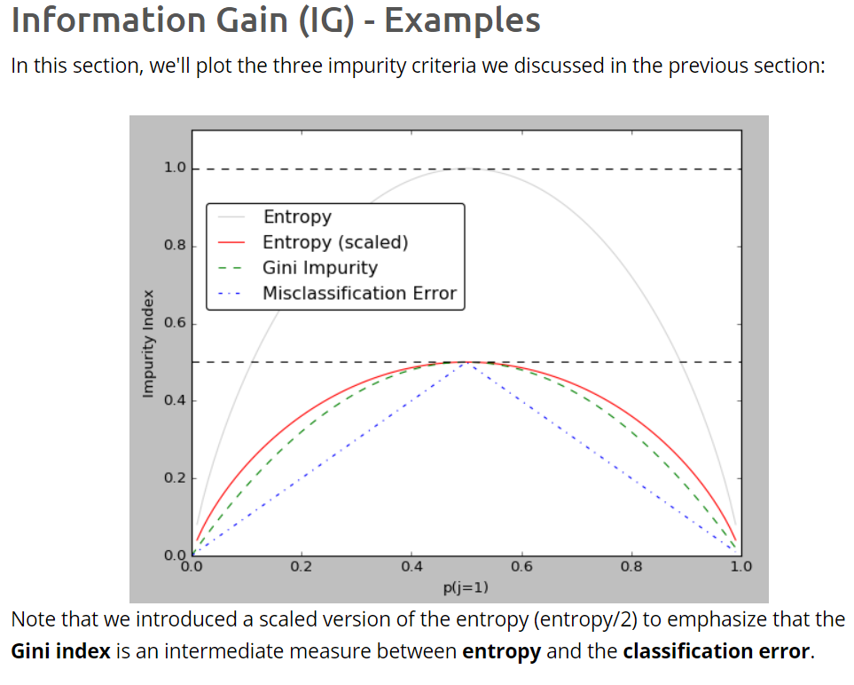
Metrics
- Gini Impurity
- Entropy
- Information Gain
Nice Meterial :
http://people.revoledu.com/kardi/tutorial/DecisionTree/how-to-measure-impurity.htm
http://www.bogotobogo.com/python/scikit-learn/scikt_machine_learning_Decision_Tree_Learning_Informatioin_Gain_IG_Impurity_Entropy_Gini_Classification_Error.php
Algorithms for constructing decision trees usually work top-down a variable at each step that best splits the set of items. Different algorithms use different metrics for measuring "best". These generally measure the homogeneity of the target within the subsets. some examples are given above.
1. Gini Impurity
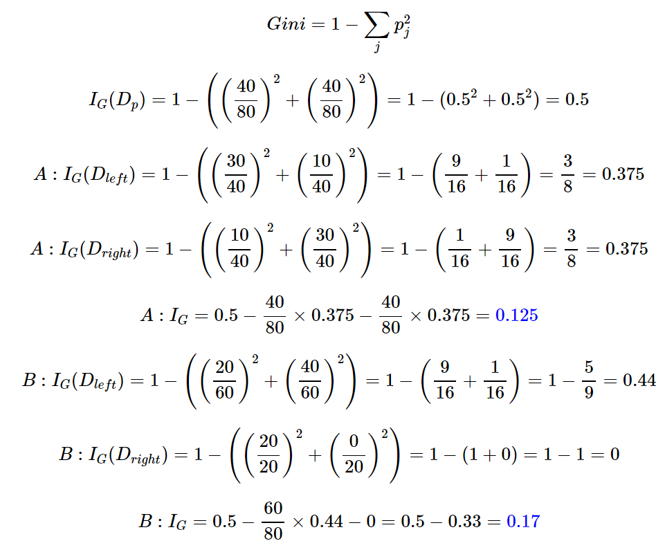
Used by the CART algorithm for classification trees, Gini impurity is a measure of how often a randomly chosen element from the set would be incorrectly labelled if it was randomly labelled according to the distribution of labels in the subset. The Gini impurity can be computed by summing the probability $p_i$ of an item with label $i$ being chosen times the probability $\sum_{k\neq i}p_k = 1 - p_i$ of a mistake in categorising that item. It reaches its minimum when all cases in the node fall into a single target category.
To compute Gini impurity for a set of items with $J$ classes, suppose $i\in$ {$1,2,...,J$}, and let $p_i$ be the fraction of items labelled with class $i$ in the set.
I_G(p) = \sum^J_{i=1}p_i \sum_{k \neq i}p_k = \sum^J_{i=1} p_i(1-p_i) = \sum^J_{i=1}(p_i - p_i)^2 = 1 - \sum^J_{i=1}p_i^2
2. Entropy : wikipedia
The basic idea of information theory is the more one knows about a topic, the less new information one is apt to get about it. If an event is very probable, it is no surprise when it happens and thus provides little new information. Inversely, if the event was improbable, it is much more informative that the event happened. Since the measure of information entropy associated with each possible data value is the negative logarithm of the probability mass function for the value, when the data source has a lower-probability value, the event carries more "information" than when the source data has a higher-probability value.
H(X) = E[I(X)] = E[-ln(P(x))]\\
H(X) = \sum^n_{i=1}P(x_i)I(x_i) = -\sum^n_{i=1}P(x_i)logP(x_i)
3. Information Gain
Using a decision tree algorithm, we start at the tree root and split the data on the feature that results in the largest information gain(IG).
We repeat this splitting procedure at each child node down to the empty leaves. this means that the samples at ach node all belong to the same class.
However, this can result in a very deep tree with many nodes, which can easily lead to overfitting. Thus, we typically want to prune the tree by setting a limit for the maximum depth of the tree.
Basically, using IG, we want to determine which attribute in a given set of training feature vectors is most useful. In other words, IG tells us how important a given attribute of the feature vector is.
We will use it to decide the ordering of attributes in the nodes of a decision tree.
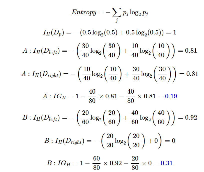
IG can be defined as follows:
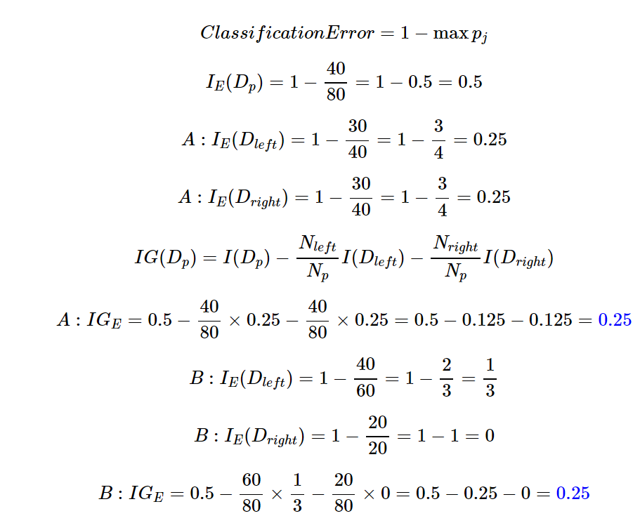
IG(D_p) = I(D_p) - \frac{N_{left}}{N_p}I(D_{left}) - \frac{N_{right}}{N_p}I(D_{right})
where $I$ could be entropy, Gini index, classification error.
Example(IG) : Reference
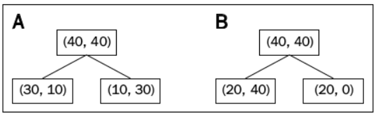
IG with Classification Error
IG with Gini Index
IG with Entropy
Usage
print(__doc__)
import numpy as np
import matplotlib.pyplot as plt
from sklearn.datasets import load_iris
from sklearn.tree import DecisionTreeClassifier
# Parameters
n_classes = 3
plot_colors = "ryb"
plot_step = 0.02
# Load data
iris = load_iris()
for pairidx, pair in enumerate([[0, 1], [0, 2], [0, 3],
[1, 2], [1, 3], [2, 3]]):
# We only take the two corresponding features
X = iris.data[:, pair]
y = iris.target
# Train
clf = DecisionTreeClassifier().fit(X, y)
# Plot the decision boundary
plt.subplot(2, 3, pairidx + 1)
x_min, x_max = X[:, 0].min() - 1, X[:, 0].max() + 1
y_min, y_max = X[:, 1].min() - 1, X[:, 1].max() + 1
xx, yy = np.meshgrid(np.arange(x_min, x_max, plot_step),
np.arange(y_min, y_max, plot_step))
plt.tight_layout(h_pad=0.5, w_pad=0.5, pad=2.5)
Z = clf.predict(np.c_[xx.ravel(), yy.ravel()])
Z = Z.reshape(xx.shape)
cs = plt.contourf(xx, yy, Z, cmap=plt.cm.RdYlBu)
plt.xlabel(iris.feature_names[pair[0]])
plt.ylabel(iris.feature_names[pair[1]])
# Plot the training points
for i, color in zip(range(n_classes), plot_colors):
idx = np.where(y == i)
plt.scatter(X[idx, 0], X[idx, 1], c=color, label=iris.target_names[i],
cmap=plt.cm.RdYlBu, edgecolor='black', s=15)
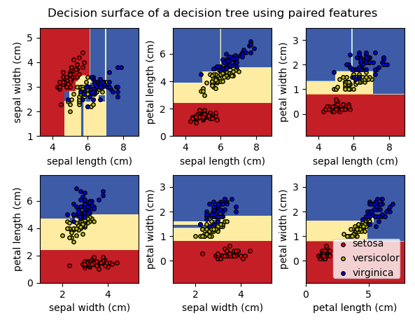
plt.suptitle("Decision surface of a decision tree using paired features")
plt.legend(loc='lower right', borderpad=0, handletextpad=0)
plt.axis("tight")
plt.show()
print(__doc__)
# Import the necessary modules and libraries
import numpy as np
from sklearn.tree import DecisionTreeRegressor
import matplotlib.pyplot as plt
# Create a random dataset
rng = np.random.RandomState(1)
X = np.sort(5 * rng.rand(80, 1), axis=0)
y = np.sin(X).ravel()
y[::5] += 3 * (0.5 - rng.rand(16))
# Fit regression model
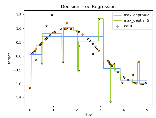
regr_1 = DecisionTreeRegressor(max_depth=2)
regr_2 = DecisionTreeRegressor(max_depth=5)
regr_1.fit(X, y)
regr_2.fit(X, y)
# Predict
X_test = np.arange(0.0, 5.0, 0.01)[:, np.newaxis]
y_1 = regr_1.predict(X_test)
y_2 = regr_2.predict(X_test)
# Plot the results
plt.figure()
plt.scatter(X, y, s=20, edgecolor="black",
c="darkorange", label="data")
plt.plot(X_test, y_1, color="cornflowerblue",
label="max_depth=2", linewidth=2)
plt.plot(X_test, y_2, color="yellowgreen", label="max_depth=5", linewidth=2)
plt.xlabel("data")
plt.ylabel("target")
plt.title("Decision Tree Regression")
plt.legend()
plt.show()