Foreword
Autoencoders play a key role in deep neural network architectures for transfer learning and other tasks.
By analytically investigating the architecture of autoencoder, it leads us to certain general framework.
And in fact, learning the framework of autoencoder sheds the light on the understanding of deep architectures.
So in this article, I would like to review the research paper below.
Title: Autoencoders, Unsupervised Learning, and Deep Architectures
Author: Pierre Baldi
Publish Year: 2012
Link: http://proceedings.mlr.press/v27/baldi12a/baldi12a.pdf
My implementation
Introduction
Initially autoencoder was invented by the collaborative work of Hinton and PDP group(Rumelheart) in 1986.
Recently it has got huge attention again because of the new discovery of the powerful architecture, which is a variational encoder.
The aim of this paper is to derive a better theoretical understanding of autoencoders and get a good insight of the nature of deep architectures.
A general Autoencoders Framework
Let us define the settings related with the framework in advance and then move on to the explanation of the architecture of it.
| name | notation |
|---|---|
| weight matrix: n->p | B |
| weight matrix: p->n | A |
| Input/Target | $X = ${$x_1, . . . , x_m$} |
| Target *optional | $Y = ${$y_1, . . . , y_m$} |
| Dissimilarity | $\Delta$ |

So the main purpose of autoencoder is, again, to obtain a meaningful representation of the dataset, so we want a model to have a strong reproducibility.
Based on the settings above, I would like to build the mathematical equations below.
min \space E(A,B) = min_{A,B} \space \sum^m_{t=1} E(x_t) = min_{A,B} \space \sum^m_{t=1} \Delta(A o B(x_t), x_t)
Case: non auto-associative
min \space E(A,B) = min_{A,B} \space \sum^m_{t=1} E(x_t, y_t) = min_{A,B} \space \sum^m_{t=1} \Delta(A o B(x_t), y_t)\\
Simply saying...
The basic autoencoder is describe as below.
- Input -> Hidden
$y = f(W^Tx + b)$ where f is some activation function e.g. sigmoid/ReLU/Tanh... - Hidden -> Output
$z = f(W'^Tz + b)$ where f is some activation function e.g. sigmoid/ReLU/Tanh... - Cost Function: Cross Entropy loss function
$L(x,z) = H(B_x || B_y) = -\sum^d_{k=1} y_k \log z_k$
And if we backpropagate the error from the output layer through the net, then it can learn how to reproduce the input.
So the important part is not the generated output, but the weight matrix. Because while it learns, it squashes the features into weight matrix in numerical format.
More interesting way to understand the architecture is below's image.
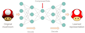
image source: http://curiousily.com/data-science/2017/02/02/what-to-do-when-data-is-missing-part-2.html
Problem in Autoencoder
So as we have seen above, the mathematically this ability of representing the dataset is proved. But there remains the problem, which is that it tends to learn Identity Function.
Hence, it is not robust anymore. I have prepared the explanatory image of this phenomena below.
 Source: https://stats.stackexchange.com/questions/130809/autoencoders-cant-learn-meaningful-features
keras implementation
Following this great post
https://blog.keras.io/building-autoencoders-in-keras.html
Dataset: mnist images => Train:(60000, 784) Test:(10000, 784)
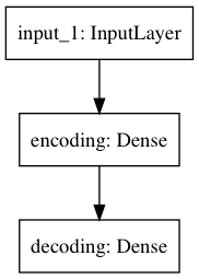
Architecture:
_________________________________________________________________
Layer (type)                 Output Shape              Param #
=================================================================
input_1 (InputLayer)         (None, 784)               0
_________________________________________________________________
encoding (Dense)             (None, 32)                25120
_________________________________________________________________
decoding (Dense)             (None, 784)               25872
=================================================================
Total params: 50,992
Trainable params: 50,992
Non-trainable params: 0
_________________________________________________________________
Code
from keras.layers import Input, Dense
from keras.models import Model

# building a model
encoding_dim = 32

input_img = Input(shape=(784, ))
encoded = Dense(encoding_dim, activation='relu', name='encoding')(input_img)
decoded = Dense(784, activation='sigmoid', name='decoding')(encoded)
autoencoder = Model(input_img, decoded)
encoder = Model(input_img, encoded)
encoded_input = Input(shape=(encoding_dim, ))
decoded_layer = autoencoder.layers[-1]
decoder = Model(encoded_input, decoded_layer(encoded_input))
autoencoder.compile(optimizer='adam', loss='binary_crossentropy')

# summariseing the model architecture
autoencoder.summary()

# save the architecture in image
from keras.utils import plot_model
plot_model(autoencoder, to_file='model.png')

# get and prepare dataset
from keras.datasets import mnist
import numpy as np
(x_train, _), (x_test, _) = mnist.load_data()

x_train = x_train.astype('float32') / 255.
x_test = x_test.astype('float32') / 255.
x_train = x_train.reshape((len(x_train), np.prod(x_train.shape[1:])))
x_test = x_test.reshape((len(x_test), np.prod(x_test.shape[1:])))
print(x_train.shape, x_test.shape)

# fit the model to the dataset
autoencoder.fit(x_train, x_train, epochs=2, batch_size=256, shuffle=True, validation_data=(x_test, x_test))

# saving the model in a format of serialize weights to HDF5
autoencoder.save_weights("model.h5")
print("Saved model to disk")

# presentation part: try reproducing the image to see how it worked
encoded_imgs = encoder.predict(x_test)
decoded_imgs = decoder.predict(encoded_imgs)

# showing the image
import matplotlib.pyplot as plt

n = 10
plt.figure(figsize=(20, 4))
for i in range(n):
	ax = plt.subplot(2, n, i+1)
	plt.imshow(x_test[i].reshape(28, 28))
	plt.gray()
	ax.get_xaxis().set_visible(False)
	ax.get_yaxis().set_visible(False)

	# display reconstruction
	ax = plt.subplot(2, n, i + 1 + n)
	plt.imshow(decoded_imgs[i].reshape(28, 28))
	plt.gray()
	ax.get_xaxis().set_visible(False)
	ax.get_yaxis().set_visible(False)
plt.show()
Learning Result
 I found that even in a few epochs, this model can achieve certain work.
Although this embeddings are really sparse matrix, the computational efficiency was retained on my machine.
I found that even in a few epochs, this model can achieve certain work.
Although this embeddings are really sparse matrix, the computational efficiency was retained on my machine.
Future Work
Since I have learned the pros and cons of autoencoders through the reviewing the paper, I would like to know how to solve the issue. In fact, there is already advanced research on this point and created the model for this as well.
So I will review that paper soon.