contents
- Introduction
- Finite Difference Policy Gradient
- Monte-Carlo Policy Gradient
- Actor-Critic Policy Gradient
1. Introduction
At first, let's look back what we have learned at last lecture.
Look-back
Last Lecture:
- Approximation of value functions or action-value functions using parameters $\theta$.
V_{\theta}(s) \approx V^π(s)\\
Q_{\theta}(s, a) \approx Q^π(s, a)
- A policy was generated directly from the value function using $\epsilon$greedy policy.
But, in this lecture, we will straightly parametrise the policy with adaptation of new methodology named Actor-Critic.
$π_{\theta}(s, a) = P[a | s, \theta]$
Overview of value-based and policy-based RL
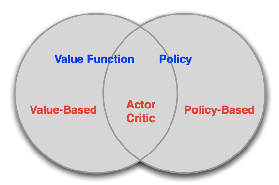 So simply saying, value-based approaches are learning value function, e.g. $\epsilon$greedy method
On the other hand, policy-based approaches rely on no value functions, instead on policy. And lastly, you must notice the beforementioned new method named Actor-Critic approach is learning value function and policy. It is like a hybrid model.
So simply saying, value-based approaches are learning value function, e.g. $\epsilon$greedy method
On the other hand, policy-based approaches rely on no value functions, instead on policy. And lastly, you must notice the beforementioned new method named Actor-Critic approach is learning value function and policy. It is like a hybrid model.
Pros/Cons of Policy-Based RL
Policy-based RL allows us to be more simple, while the value function contains and relates to other complicated concepts. I have summarised the advantages and disadvantages.
Advantages
- Better convergence properties
- Effective in high-dimensional or continuous action spaces
- Being able to learn stochastic policies
Disadvantages
- Can converge to a local minimum rather than global optimum
- Evaluating policy is generally inefficient and high variance(oscillating)
Comparison of Value/Policy based RL
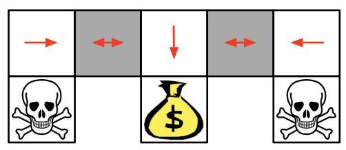
Firstly think about the game setting. We consider the gridworld problem named Alised GridWorld. Starting points, which are at the bottom corners, are marked by a bit scary skulls.
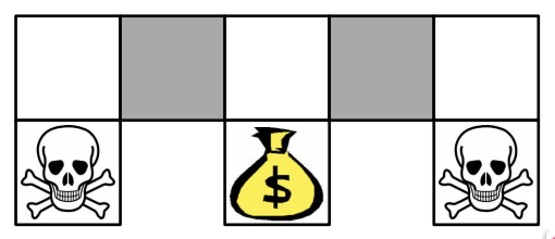
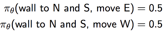
And the agent is not able to distinguish grey areas. So based on this game, we can come up with two models described below.
PotenialActions: \phi(s,a) = 1(North,East,South,West)\\
Value Based RL: Q_{\theta}(s,a) = f(\phi(s,a), \theta)\\
Policy BasedRL: π_{\theta}(s,a) = g(\phi(s,a), \theta)
Hence, we could see significant difference in the result between these two methods.
Value-Based RL
this method keep picking deterministic policy, so it can get stuck in either grey area as you can see below.
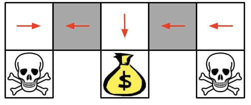
Although, we can adapt $\epsilon$greedy approach, still it takes time comparing to policy-based RL.
Policy-Based RL
As you can see that the model will reach the goal state in a few steps with high probability, and it's much faster than value-based RL.
Policy Search
So far, we have confirmed that the policy-based RL is much preferable than value-based RL in some situations. So, let's dig policy-based RL more.
In this section, I would like to write about the way to measure the quality of policies. In fact, there are three methods to scale the policy.
1.Start value:
J_1(\theta) = V^{π_{\theta}}(s_1) = E_{π_{\theta}}[v_1]
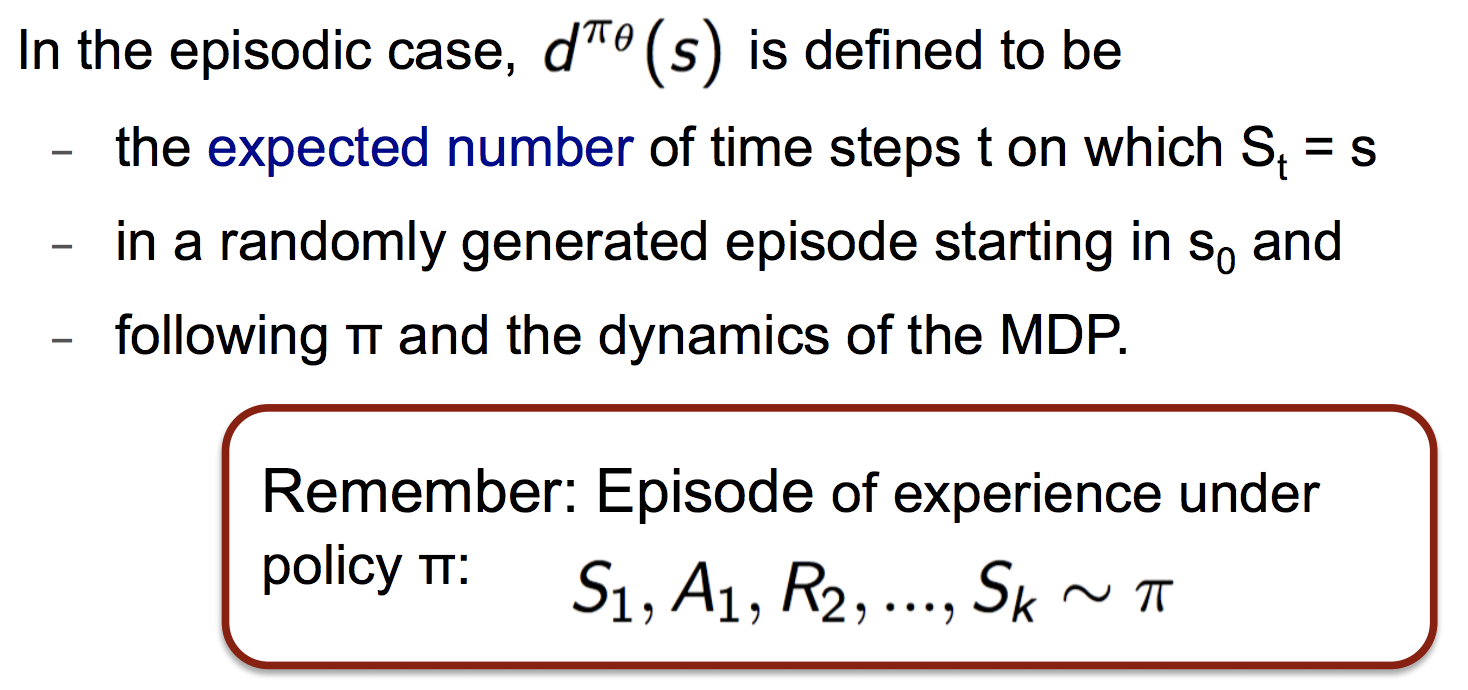
2.Average value:
J_{avV}(\theta) = \sum_s d^{π_{\theta}}(s) V^{π_{\theta}}(s)
3.Average reward per time-step
J_{avR}(\theta) = \sum_s d^{π_{\theta}}(s) \sum_a π_{\theta}(s,a) R^a_s\\
where \space d^{π_{\theta}}(s) \space is \space stationary \space distribution \space of \space Markov \space chain \space for \space π_{\theta}
from this PPT, there is another explanation here.
http://www.cs.cmu.edu/~rsalakhu/10703/Lecture_PG.pdf
Policy Gradient Ascent
Based on what we have seen in previous section, we could define the objective functions for optimisation.
So in this section, I would like to write about the method to reach the optimum by tuning parameters contained in those objective functions.
As you probably know, the gradient ascend algorithms for searching local maximum in objective function(cost/loss).
** this is really good explanation on the difference between loss, cost and objective functions
A loss function is a part of a cost function which is a type of an objective function.
Hence, let me brief the appearance of gradient ascent first, then move on to the details of Policy gradient.
\Delta \theta = \alpha \nabla_{\theta}J(\theta)\\
\nabla_{\theta}J(\theta) = \left(
\begin{matrix}
\frac{\partial J(\theta)}{\partial \theta_1} \\
\vdots \\
\frac{\partial J(\theta)}{\partial \theta_n}
\end{matrix}
\right)\\
\alpha = step size
So let's move on to the actual procedure of calculation.
Indeed, we have two options,
- Get job done... => do partial derivative w.r.t all parameters in the objective function.
- Naive approach
Assuming that you are able to work hard by calculating one by one anyhow, like using python we could define the derivative of objective function and use outer product to apply it to the weight matrix, so I would like to talk about the second option from now.
We traverse the dimensions described $k \in [1,n]$ and apply partial derivative w.r.t each $\theta$.
\frac{\partial J(\theta)}{\partial \theta_k} \approx \frac{\partial J(\theta + \epsilon u_k) - J(\theta)}{\epsilon}
This one is actually noisy a bit, but helpful in case where the objective function is not differentiable.
Monte-Carlo Policy Gradient
Likelihood Ratios
reference web-site
Likelihood ratios (LR) in medical testing are used to interpret diagnostic tests. Basically, the LR tells you how likely a patient has a disease or condition. The higher the ratio, the more likely they have the disease or condition. Conversely, a low ratio means that they very likely do not. Therefore, these ratios can help a physician rule in or rule out a disease.
We now compute the policy gradient analytically.
Assuming that policy is differentiable whenever it is non-zero, and $\nabla_{\theta}π_{\theta}(s,a)$ denotes the gradient of policy.
We could describe likelihood ratios as below.
Based \space on \space chain \space rule.\\
\nabla_{\theta} π_{\theta}(s,a) = π_{\theta}(s,a) \frac{\nabla_{\theta}π_{\theta}(s,a)}{π_{\theta}(s,a)}\\
= π_{\theta}(s,a) \nabla_{\theta} \log π_{\theta}(s,a)
And the score function is : $\nabla_{\theta} \log π_{\theta}(s,a)$
Softmax Policy
So, as a sample, we are going to see softmax policy.
What this does is simple, we weight actions using linear combination: $\phi(s,a)^T\theta$.
And then to estimate the probability for each action, we will apply softmax function. $\pi_{\theta}(s,a_n) \approx \frac{e^{\phi(s,a_n)^T\theta}}{\sum_k e^{\phi(s,a_k)^T\theta} } \space for \space all \space possible \space actions $
The score function is:
\nabla_{\theta} \log π_{\theta}(s,a) = \phi(s,a) - E_{\pi_{\theta}}[\phi(s,a)]
Gaussian Policy
When the action is distributed in continuous space, then Gaussian method is fitting.
Mean: $\mu(s) = \phi(s)^T\theta$
Variance: can be either $\sigma^2$ or parametrised.
Since, policy is gaussian, then potential actions will be sampled from Gaussian Distribution. $a \sim N(\mu(s), \sigma^2)$
The score function is:
\nabla_{\theta} \log π_{\theta}(s,a) = \frac{(a - \mu(s))\phi(s)}{\sigma^2}
One-step MDP
So far, we have understood how we could form the parametrised policy and quote the score functions from it.
In this section, let's go practical a bit, we are going to consider a "One-step MDPs".
Start state: $s \sim d(s)$
Reward after one-step: $r = R_{s,a}$
Using likelihood ratios to compute the policy gradient,
\begin{align}
J(\theta) &= E_{\pi_{\theta}}[r]\\
&= \sum_{s \in S}d(s) \sum_{a \in A} \pi_{\theta}(s,a)R_{s,a}\\
\nabla_{\theta}J(\theta) &= \sum_{s \in S}d(s) \sum_{a \in A} \pi_{\theta}(s,a) \nabla_{\theta} \log π_{\theta}(s,a) R_{s,a} \\
 &= E_{\pi_{\theta}}[\log π_{\theta}(s,a) r]
\end{align}
Policy Gradient Theorem
Hereby, we have become familiarised with any forms of policies, like softmax/gaussian using score functions based on likelihood ratios approach.
So, let's theorise policy gradient in this section.
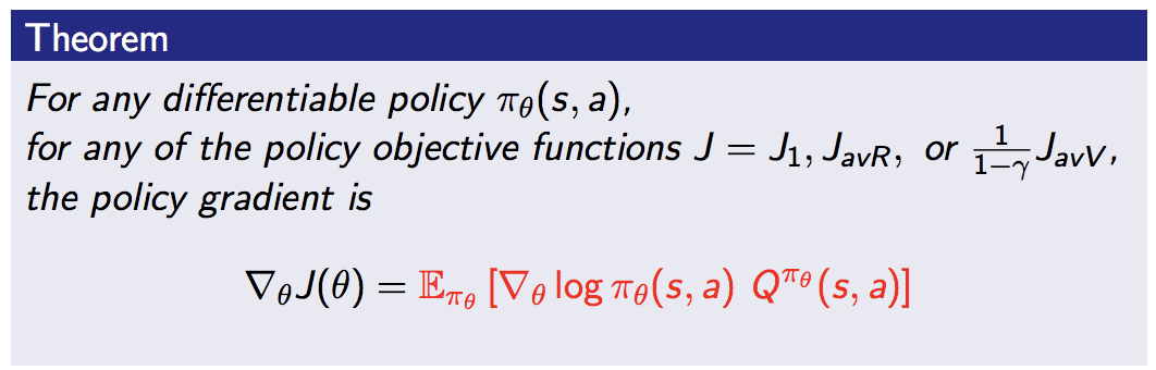
** we replace instantaneous reward $r$ with long term action-value function $Q^{π_{\theta}}(s,a)$ which is unbiased sample. And policy gradient should be combined with objective functions as we saw before.
Let's see the simple example using Monte-Carlo.
Monte-Carlo Policy Gradient(Func name is REINFORCE)
As a running example, I would like to show the algorithmic function equipped with policy gradient method.
First of all, let me configure the situation, we update parameters by SGD and use policy gradient ofcourse.
So simply formulating,
\Delta \theta_t = \alpha \nabla_{\theta}\log π_{\theta}(s_t, a_t)Q^{π_{\theta}}(s_t, a_t)
where \space v_t = Q^{π_{\theta}}(s_t, a_t)

Actor-Critic Algorithm
Finally, we have come to this topic. As a matter of fact, monte-carlo policy gradient contains high variance because as we leaned in some statistics class a sample is just a randomly selected example from the population. Hence, every episode we go through, the value of a sample would vary. So to decrease variance, we want to estimate a distribution samples belong to.
Good review of stats: http://www.statisticshowto.com/sample-variance/
I would like to adapt new concept which is a critic to estimate the action-value function.
$Q_w(s,a) \approx Q^{\pi_{\theta}}(s,a)$
Frankly speaking, actor critic algorithm maintain two sets of parameters
- Critic: updates action-value function(the one related the action which actor takes) parameters, $w$
- Actor: updates policy parameters $\theta$, in direction suggested by critic.
\nabla_{\theta}J(\theta) \approx E_{\pi_{\theta}}[\nabla_{\theta} \log \pi_{\theta}(s,a) Q_w(s,a)]\\
\Delta \theta = \alpha \nabla_{\theta} \log \pi_{\theta}(s,a) Q_w(s,a)
In fact, critic evaluates the policy using the algorithms we saw already, like TD/MC and least-squares policy evaluation so on.
So to grab the overview, let's see a use case.
Critic: updates $w$ by linear TD(0)
Actor: updates $\theta$ by policy gradient
Using linear value function approximation: $Q_w(s,a) \approx \phi(s,a)^Tw$
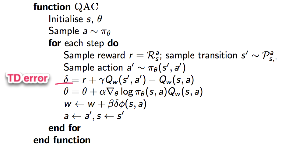 Notation:
step-sizes: $\alpha, \beta$ => indicating how much you are greedy, if those are 1, then just a greedy policy.
Notation:
step-sizes: $\alpha, \beta$ => indicating how much you are greedy, if those are 1, then just a greedy policy.
So the important thing here is that since we update $\theta$ step by step we are approaching optimal policy step by step.
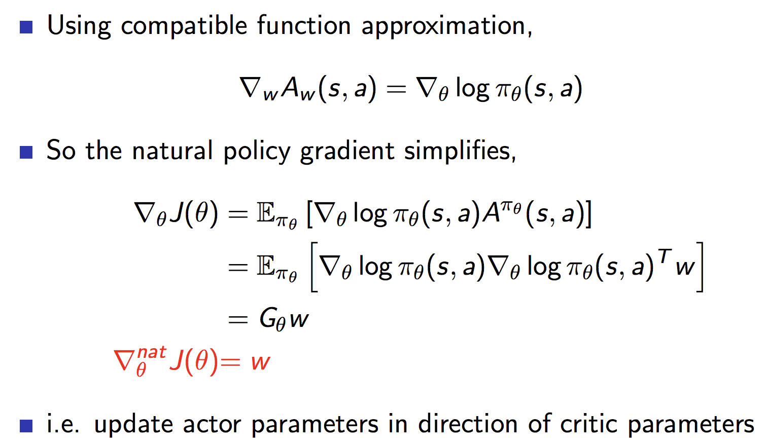
Compatible Function Approximation
Good reference:
- https://datascience.stackexchange.com/questions/25259/what-is-compatible-function-approximation-theorem-in-reinforcement-learning
- https://papers.nips.cc/paper/1713-policy-gradient-methods-for-reinforcement-learning-with-function-approximation.pdf
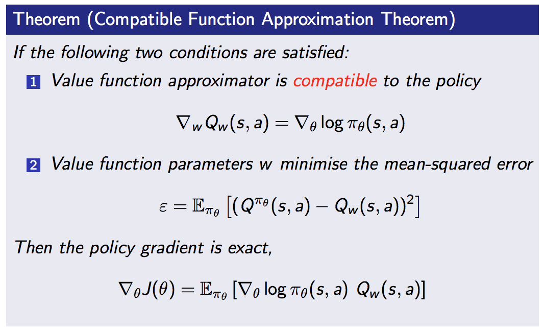
And let's see the mathematical proofs.
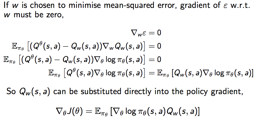
Based on this theory, we could confirm that $Q_w(s,a) = Q^{\pi_{\theta}}(s,a)$
By the way, we haven't thought about the way to reduce the variance yet in Actor-Critic Algorithm as I mentioned at the beginning of this topic, so let's check that out for now!.
Reducing Variance Using a Baseline ~ Advantage Function Critic ~
By subtracting a baseline function $B(s)$ from the policy gradient, we can reduce the variance, without changing expectation.
\begin{align}
E_{\pi_{\theta}}[\nabla_{\theta} \log \pi_{\theta}(s,a)B(s)] &=  \sum_{s \in S}d^{\pi_{\theta}}(s) \sum_a \nabla_{\theta}\pi_{\theta}(s,a)B(s)\\
&= \sum_{s \in S}d^{\pi_{\theta}}(s) B(s) \nabla_{\theta} \sum_a \pi_{\theta}(s,a)\\
&= 0
\end{align}
In fact, a good baseline equates the state value function $B(s) = V^{\pi_{\theta}}(s)$
So we can rewrite the policy gradient using the Advantage Function $A^{\pi_{\theta}}(s,a)$
A^{\pi_{\theta}}(s,a) = Q^{\pi_{\theta}}(s,a) - V^{\pi_{\theta}}(s)\\
\nabla_{\theta}J(\theta) = E_{\pi_{\theta}}[\nabla_{\theta} \log \pi_{\theta}(s,a)A^{\pi_{\theta}}(s,a)]
Hence, we can significantly reduce the variance of policy gradient with the advantage function though, ofcourse we need to estimate two functions contained the advantage function.
V_v(s) \approx V^{\pi_{\theta}}(s)\\
Q_w(s,a) \approx Q^{\pi_{\theta}}(s,a)\\
A(s,a) = Q_w(s,a) - V_v(s)
However, as you might understand already using two parameters to estimate two functions can be turning out a quite poor result. Hence, we tend to rely on TD-Error and so on.
Estimating the Advantage Function ~ TD-Error example ~
First of all, we assume that for the true value function $V^{\pi_{\theta}}(s)$, the TD error $\delta^{\pi_{\theta}}$ is an unbiased estimate of the advantage function.
\delta^{\pi_{\theta}} = r + \gamma V^{\pi_{\theta}}(s')  - V^{\pi_{\theta}}(s) \\

\begin{align}
E_{\pi_{\theta}}[\delta^{\pi_{\theta}} | s,a] &= E_{\pi_{\theta}}[r + \gamma V^{\pi_{\theta}}(s') | s,a] - V^{\pi_{\theta}}(s)\\
&= Q^{\pi_{\theta}}(s,a) - V^{\pi_{\theta}}(s)\\
&= A^{\pi_{\theta}}(s,a)
\end{align}
Hence, with TD error, the policy gradient will be like below
\nabla_{\theta}J(\theta) = E_{\pi_{\theta}}[\nabla_{\theta} \log \pi_{\theta}(s,a)
 \delta^{\pi_{\theta}}]
So in this equation, we need a parameter.
Likewise, we can apply this technique to the algorithms we have seen ever.
Let's see it from two angles, which is critics aspect and actors aspect respectively.
Critics at Different Time-Scales
- For MC, the target is the return $v_t$,
$\Delta \theta = \alpha(v_t - V_{\theta}(s))\phi(s)$ - For TD(0), the target is the TD target $r + \gamma V(s')$,
$ \Delta \theta = \alpha(r + \gamma V(s') - V_{\theta}(s))\phi(s) $ - For forward-view TD($\lambda$), the target is the $\lambda$ return $v_t^{\lambda}$,
$ \Delta \theta = \alpha(v_t - V_{\theta}(s))\phi(s) $ - For backward-view TD($\lambda$), we use eligibility traces
\delta_t = r_{t+1} + \gamma V(s_{t+1}) - V(s_t)\\
e_t = \gamma \lambda e_{t-1} + \phi(s_t)\\
\Delta \theta = \alpha \delta_t e_t
Actors at Different Time-Scales

Natural Gradient

Fisher Information
from wikipedia
In mathematical statistics, the Fisher information (sometimes simply called information[1]) is a way of measuring the amount of information that an observable random variable X carries about an unknown parameter θ of a distribution that models X. Formally, it is the variance of the score, or the expected value of the observed information. In Bayesian statistics, the asymptotic distribution of the posterior mode depends on the Fisher information and not on the prior (according to the Bernstein–von Mises theorem, which was anticipated by Laplace for exponential families).[2] The role of the Fisher information in the asymptotic theory of maximum-likelihood estimation was emphasized by the statistician Ronald Fisher (following some initial results by Francis Ysidro Edgeworth). The Fisher information is also used in the calculation of the Jeffreys prior, which is used in Bayesian statistics.
Good reference:
http://people.missouristate.edu/songfengzheng/Teaching/MTH541/Lecture%20notes/Fisher_info.pdf
https://web.stanford.edu/class/stats311/Lectures/lec-09.pdf