① 勉強テーマ
ニューラルネットワークが深層学習へと進化していく過程
② 勉強の背景
自習の一環として、これまで深層学習のことを勉強をしてきたが、それがどういった問題から生じてきた手法であったのかの原点に立ち返ることが必要であると感じたので
③ 勉強の方法
こちらのリンクに掲載をしていただいている著者の素晴らしいリソースを拝借いたします
http://nnadl-ja.github.io/nnadl_site_ja/chap1.html
④ 期待される成果
深層学習の生まれたきっかけをつかみ、根本的な問題解決の新しい方法を見つけること
GITHUB: https://github.com/Rowing0914/NeuralNetwork_DeepLearning
構成
- イントロダクション
- パーセプトロン
- シグモイドニューロン
- ニューラルネットワークのアーキテクチャ
- 手書き数字を分類する単純なネットワーク
- 勾配降下法を用いた学習
- 手書き数字を分類するニューラルネットワークの実装
- Deep Learning に向けて
1. イントロダクション
この章では手書き数字認識を学習するニューラルネットワークを実装することを目標とする。
それを学ぶ過程で深層学習へと至る重要なテクニックのいくつかをみていく。
2. パーセプトロン
ニューラルネットワークの誕生に先立ち、人口ニューロン(パーセプトロンetc)から話を開始する。
パーセプトロンは、1950年代から1960年代にかけて、 Warren McCullochと Walter Pittsらの 先行研究に触発された Frank Rosenblattによって 開発された。
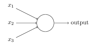
output = \left\{
\begin{array}{ll}
1 & if \sum_j w_jx_j \leq threshold \\
0 & if \sum_j w_jx_j > threshold
\end{array}
\right.
直感的理解
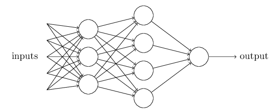
複数の情報に重み($w$)をつけながら決定を下す機械である。
これを複数の層に重ねると、多層のニューラルネットワークとなり、より高度な判断を下せるようになる。
output = \left\{
\begin{array}{ll}
1 & if \sum_j wx+b \leq threshold \\
0 & if \sum_j wx+b > threshold
\end{array}
\right.
直感的理解
バイアスとはニューロンが発火する時の傾向の高さを表すものと言える。
この閾値を超えると発火をするから。
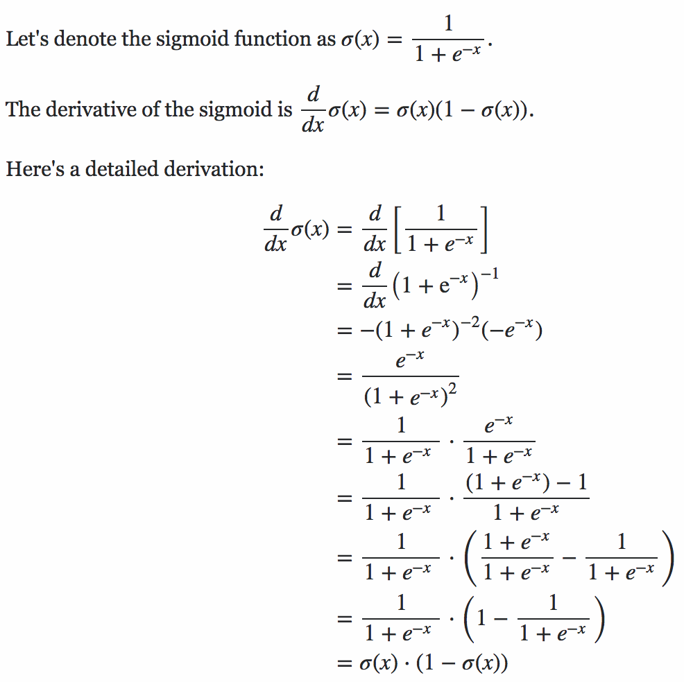
3. シグモイドニューロン
シグモイド関数
\sigma(z) = \frac{1}{1+e^{-z}}\\
\sigma(z) = \frac{1}{1+exp(-\sum_jw_jx_j - b)}
実装
import numpy as np
import matplotlib.pyplot as plt

def sigmoid(a):
	res = []
	for e in a:
		res.append(1/(1+np.exp(-e)))
	return res

a = list(range(-20,20,1))
print(sigmoid(a))

plt.plot(sigmoid(a))
plt.show()
\Delta output \approx \sum_j \frac{\delta output}{\delta w_j}\Delta w_j + \frac{\delta output}{\delta b_j}\Delta b_j
直感的理解
outputの偏微分をして、全ての重み$w_j$の和、をそれぞれにかけている、つまり、$\Delta output$は重みとバイアスにおいて、$\Delta w_j$と$\Delta x_j$の変化に対して線形であるということ、
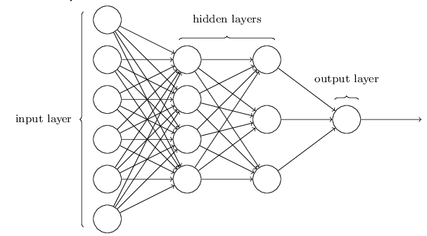
4. ニューラルネットワークのアーキテクチャ
一番左の層は入力層(input layer)と呼ばれ、その中のニューロンを入力ニューロン(input neurons)と言います。一番右の層または出力層(output layer)は、出力ニューロン(output neurons)から構成されている。
5. 手書き数字を分類する単純なネットワーク
データ
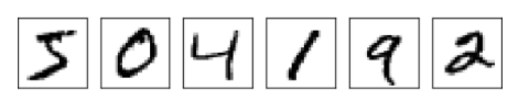
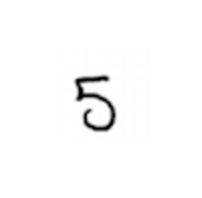
今回最初にプログラムに認識をさせるのは$5$を行いたいと思う。
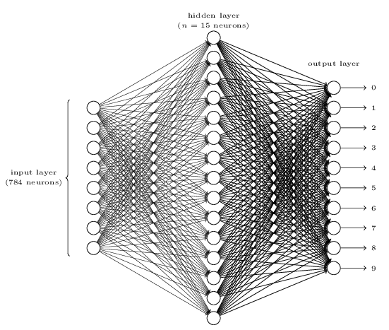
ネットワークの構成としては、少々仰々しくなってしまう。
しかし、我々が使う訓練データは28x28ピクセルの手書き数字の画像であり、この画像という元データは$28x28=784$のニューロンから構成をされると考えることができるからである。
実装:下のふざけたような5の数字の画像を使ってみてください!
import matplotlib.image as img
image = img.imread('5.png')
print(image.shape) # (402, 410, 3)
6. 勾配降下法を用いた学習
Deep Learningの父とも称されるLeCunが配布しているこちらの手書き数字の画像データを使用するとする。
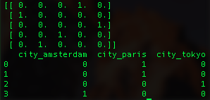
ここで、まずは、各画像を書かれている数字を元にカテゴリごとに分ける。
そした上で、各カテゴリーをベクトルで表す。
下記のコード参照。
import numpy as np
import random

n_labels = 5
_list = list(range(5))
random.shuffle(_list)
print(np.eye(n_labels)[_list])

import pandas as pd
df = pd.DataFrame(["paris", "paris", "tokyo", "amsterdam"], columns=['city'])
print(pd.get_dummies(df, columns=['city']))
Result
前半で使用した、シグモイド関数によって、数字の予測をすることができるところまでは理解が進んだ。
ここからは実際に予測をした数字と回答である数字の誤差を求めていく。
それが最終的にネットワーク内部の各判断基準を決定している重みへと伝搬されていくことにより、初期化した重みをきちんと正しいものへと昇華していくことができる。
今回は簡単のために、平均二乗誤差(MSE)を用いる。
C(w,b) = \frac{1}{2n}\sum_x|| y(x) - a ||^2
ここで w はネットワーク中の全ての重み、 b は全バイアス、 n は訓練入力の総数、 a は入力が x の時にネットワークから出力されるベクトル、和は全ての訓練入力 x である。もちろん出力 a は w と b そして x に依存しますが表記をシンプルにするためここでは敢えて明示しない。‖v‖はベクトル v の距離関数を示す記号である。要約すると、ニューラルネットワークの訓練における私たちのゴールは2次コスト関数 C(w,b) を最小化する重みとバイアスを見つけること。
では、ここからこの数式からどうやって重みの更新を行っていくのかを見ていく。
import numpy as np
import matplotlib.pyplot as plt

a = [x**2 for x in range(-10,11,1)]
plt.plot(a)
plt.show()
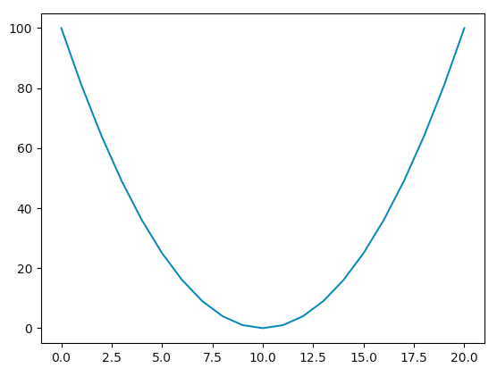
ここで実際の二次関数のグラフを参照してみる。
グラフの最小点が今回探索をしたい、コスト関数$C$を最小にする$W$の値であると言える。
今回の例は非常に単純なものであるが、数式を構成する各パラメータが何かしらの変化をすることにより、数式全体のアウトプットに影響を与える。その軌跡がこのグラフであると考えると、各パラメータをいじりながら最小の点を探すということにも納得がいくと思う。
確率的勾配降下法
訓練データからランダムに抽出した小さなサンプルに対しての$\nabla C_x$を導出して、勾配$\nabla C$を推定するというもの。
こちらのサイトにて、母集団平均とサンプル平均が一致する綺麗な証明が書かれています。
リンク
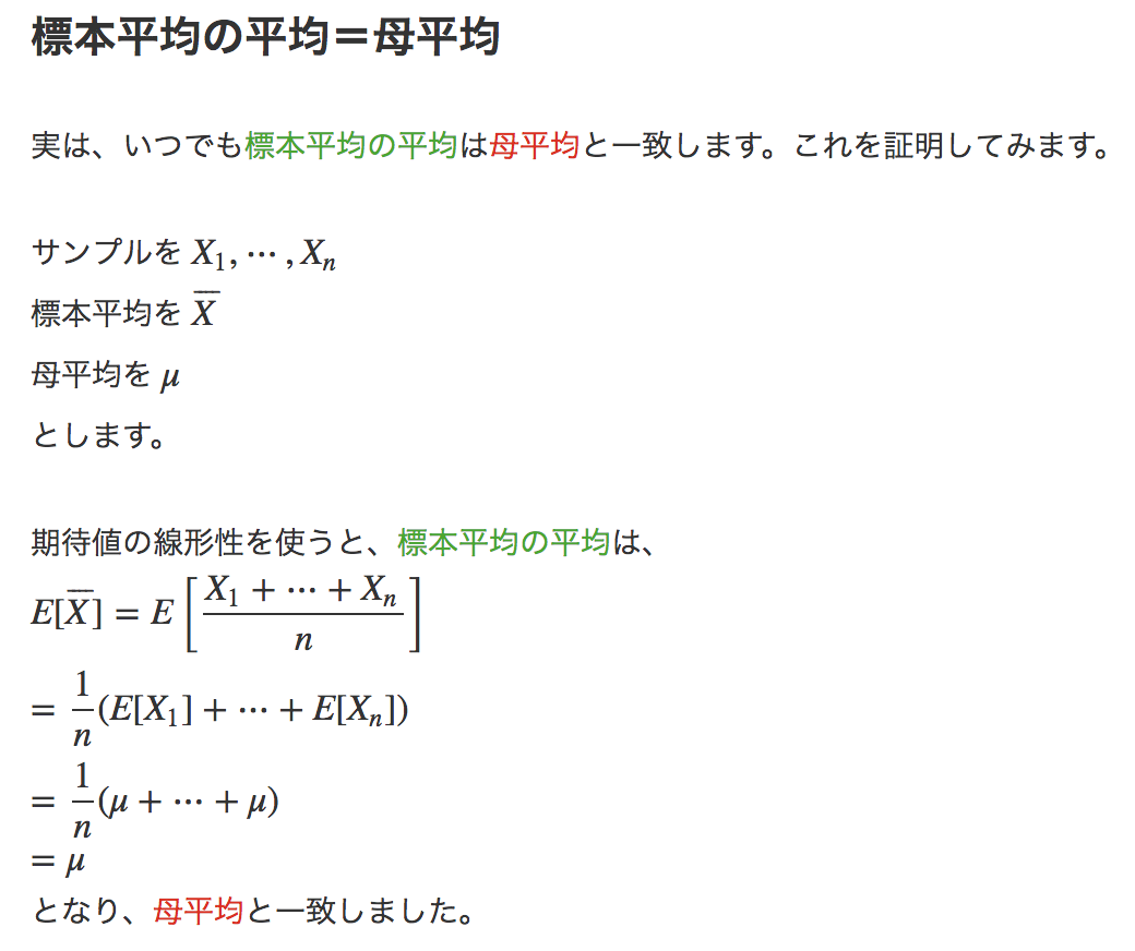
ここでこのサンプル集団を$X_1, X_2 ... X_m$をラベル付けをし、これをミニバッチと呼ぶことにする。
よって、ミニバッチを計算することが、すなわち、全体の勾配を計算することと等しいと言える。
w_k \rightarrow w'_k = w_k - \frac{\eta}{m}\sum_j \frac{\delta C_{X_j}}{\delta w_k}\\
b_l \rightarrow b'_l = b_l - \frac{\eta}{m}\sum_j \frac{\delta C_{X_j}}{\delta b_l}
であると確認ができる。これに対して、エポックという概念を導入する。エポックとは、回転数という認識が一番近いと思う。何回訓練データを回すのかを決める変数である。
つまり、各エポックごとに異なるミニバッチを元に訓練をするということだ。
7. 手書き数字を分類するニューラルネットワークの実装
まずはネットワークの初期化から見ていく。
import numpy as np
np.random.seed(42)

class Network():
	def __init__(self, sizes):
		self.num_layers = len(sizes)
		self.sizes = sizes
		self.biases = [np.random.randn(y,1) for y in sizes[1:]]
		self.weights = [np.random.randn(y,x) for x, y in zip(sizes[:-1], sizes[1:])]

	def showParams(self):
		print("number of layers: ", self.num_layers)
		print("size of network: ", self.sizes)
		print("baises: ", "\n", self.biases)
		print("weights: ","\n", self.weights)

net = Network([2,3,1])
net.showParams()

"""
OUTPUT
number of layers:  3
size of network:  [2, 3, 1]
baises:
 [array([[ 0.49671415],
       [-0.1382643 ],
       [ 0.64768854]]), array([[1.52302986]])]
weights:
 [array([[-0.23415337, -0.23413696],
       [ 1.57921282,  0.76743473],
       [-0.46947439,  0.54256004]]), array([[-0.46341769, -0.46572975,  0.24196227]])]
"""
次に、これまで見てきたSGDに関してのファンクションを見てみる。
下記に記したコードで実装が完了する。
    def sigmoid(z):
        return 1.0 / (1.0 + np.exp(-z))

    def feedforward(self, a):
        for b, w in zip(self.biases, self.weights):
            # activation layer a' = sigmoid( Wx + b )
            a = sigmoid(np.dot(w, a) + b)
        return a

    def SGD(self, training_data, epochs, mini_batch_size, eta, test_data=None):
        # training_data is a list of tuples of (X, y)
        if test_data: n_test = len(test_data)
        n = len(training_data)
        # iterate through data following the given epochs
        for j in xrange(epochs):
            # shuffle the training data
            random.shuffle(training_data)
            # create mini-batch training dataset.
            """
            [i for i in range(0, 100, 20)] => [0, 20, 40, 60, 80]
            this  means the index of mini-batch
            """
            mini_batches = [training_data[k:k + mini_batch_size] for k in xrange(0, n, mini_batch_size)]
            for mini_batch in mini_batches:
                self.update_mini_batch(mini_batch, eta)
            if test_data:
                result = float(self.evaluate(test_data))/float(n_test)
                print "Epoch {0}: {1}".format(j, result)
            else:
                print "Epoch {0} complete".format(j)
コードに説明を入れたので、実際に確認をしながら見ていってほしい。
※rangeとxrangeの違いに関して
何が異なるのかというと、大きな数を指定した時のメモリの効率です。Python 2系におけるrangeは、引数で10を指定した場合、要素を10個持つリストが作られます。これは繰り返し処理を行う前に確保されます(あらかじめ全て用意する)。これに対してxrangeはその都度必要な値を生成します。小さな要素数の場合はあまり変わりませんが、仮に10ではなく「10000000(1千万)」であった場合はどうでしょうか。一息に1千万もの要素をもつリストが作られることと、その都度必要な分だけ値を生成するのではまったく効率が異なります。なお先に述べた通りPython 3系ではxrangeはありません。rangeがxrangeに近い形へ実装し直されたため、撤廃になりました。
import numpy as np
np.random.seed(42)
import random

class Network():
    def __init__(self, sizes):
        self.num_layers = len(sizes)
        self.sizes = sizes
        self.biases = [np.random.randn(y, 1) for y in sizes[1:]]
        self.weights = [np.random.randn(y, x) for x, y in zip(sizes[:-1], sizes[1:])]

    def showParams(self):
        print("number of layers: ", self.num_layers)
        print("size of network: ", self.sizes)
        print("baises: ", "\n", self.biases)
        print("weights: ", "\n", self.weights)

    def showSizeOfParams(self):
        print("number of layers: ", self.num_layers)
        print("size of network: ", self.sizes)
        for i, (b, w) in enumerate(zip(self.biases, self.weights)):
            print("the size of biase for {0} layer: {1}".format(i+2, len(b)))
            print("the size of weight for {0} layer: {1}".format(i+2, len(w)))

    def sigmoid(z):
        return 1.0 / (1.0 + np.exp(-z))

    def feedforward(self, a):
        for b, w in zip(self.biases, self.weights):
            # activation layer a' = sigmoid( Wx + b )
            a = sigmoid(np.dot(w, a) + b)
        return a

    def SGD(self, training_data, epochs, mini_batch_size, eta, test_data=None):
        # training_data is a list of tuples of (X, y)
        if test_data: n_test = len(test_data)
        n = len(training_data)
        # iterate through data following the given epochs
        for j in xrange(epochs):
            # shuffle the training data
            random.shuffle(training_data)
            # create mini-batch training dataset.
            """
            [i for i in range(0, 100, 20)] => [0, 20, 40, 60, 80]
            this  means the index of mini-batch
            """
            mini_batches = [training_data[k:k + mini_batch_size] for k in xrange(0, n, mini_batch_size)]
            for mini_batch in mini_batches:
                self.update_mini_batch(mini_batch, eta)
            if test_data:
                result = float(self.evaluate(test_data))/float(n_test)
                print "Epoch {0}: {1}".format(j, result)
            else:
                print "Epoch {0} complete".format(j)

    def update_mini_batch(self, mini_batch, eta):
        # initialise b,w with empty list
        nabla_b = [np.zeros(b.shape) for b in self.biases]
        nabla_w = [np.zeros(w.shape) for w in self.weights]
        for x, y in mini_batch:
            delta_nabla_b, delta_nabla_w = self.backprop(x, y)
            nabla_b = [nb + dnb for nb, dnb in zip(nabla_b, delta_nabla_b)]
            nabla_w = [nw + dnw for nw, dnw in zip(nabla_w, delta_nabla_w)]
        self.weights = [w - (eta / len(mini_batch)) * nw
                        for w, nw in zip(self.weights, nabla_w)]
        self.biases = [b - (eta / len(mini_batch)) * nb
                       for b, nb in zip(self.biases, nabla_b)]

    def backprop(self, x, y):
        # initialise b, w with empty list: size in this case is [first layer: 30, second layer: 10]
        nabla_b = [np.zeros(b.shape) for b in self.biases]
        nabla_w = [np.zeros(w.shape) for w in self.weights]

        # feedforward
        activation = x
        activations = [x]  # list to store all the activations, layer by layer
        zs = []  # list to store all the z vectors, layer by layer
        for b, w in zip(self.biases, self.weights):
            # z = Wx + b
            z = np.dot(w, activation) + b
            zs.append(z)
            # sigmoid(z)
            activation = sigmoid_vec(z)
            activations.append(activation)

        # backward pass
        delta = self.cost_derivative(activations[-1], y) * sigmoid_prime_vec(zs[-1])
        nabla_b[-1] = delta
        nabla_w[-1] = np.dot(delta, activations[-2].transpose())
        # Note that the variable l in the loop below is used a little
        # differently to the notation in Chapter 2 of the book.  Here,
        # l = 1 means the last layer of neurons, l = 2 is the
        # second-last layer, and so on.  It's a renumbering of the
        # scheme in the book, used here to take advantage of the fact
        # that Python can use negative indices in lists.
        for l in xrange(2, self.num_layers):
            z = zs[-l]
            spv = sigmoid_prime_vec(z)
            delta = np.dot(self.weights[-l + 1].transpose(), delta) * spv
            nabla_b[-l] = delta
            nabla_w[-l] = np.dot(delta, activations[-l - 1].transpose())
        return (nabla_b, nabla_w)

    def evaluate(self, test_data):
        """Return the number of test inputs for which the neural
        network outputs the correct result. Note that the neural
        network's output is assumed to be the index of whichever
        neuron in the final layer has the highest activation."""
        test_results = [(np.argmax(self.feedforward(x)), y)
                        for (x, y) in test_data]
        return sum(int(x == y) for (x, y) in test_results)

    def cost_derivative(self, output_activations, y):
        """
        Return the vector of partial derivatives C_x w.r.t a for the output activations
        our case, cost func is C = (1/2)(∑||output - target||^2)
        Hence, nabla_C = (output - target)
        """
        return (output_activations - y)

if __name__ == '__main__':
    def sigmoid(z):
        """The sigmoid function."""
        return 1.0 / (1.0 + np.exp(-z))

    def sigmoid_prime(z):
        """Derivative of the sigmoid function."""
        return sigmoid(z) * (1 - sigmoid(z))

    # numpy vectorise: https://qiita.com/3x8tacorice/items/3cc5399e18a7e3f9db86
    sigmoid_vec = np.vectorize(sigmoid)
    sigmoid_prime_vec = np.vectorize(sigmoid_prime)


    import mnist_loader
    training_data, validation_data, test_data = mnist_loader.load_data_wrapper()

    net = Network([784, 30, 10])

    print(net.SGD(training_data, 1, 10, 3.0, test_data=test_data))
    net.showSizeOfParams()

"""
Epoch 0: 0.9083(accuracy)
None
('number of layers: ', 3)
('size of network: ', [784, 30, 10])
the size of biase for 2 layer: 30
the size of weight for 2 layer: 30
the size of biase for 3 layer: 10
the size of weight for 3 layer: 10
"""
長くなってしまったにもかかわらず、読んでいただきましてありがとうございました。
是非とも、実際の元記事もご覧いただけますと本記事の至らない点を誤認識いただけますと思いますので、
ご指摘いただけますと幸いです。