contents
- Introduction
- Incremental Methods
- Batch Methods
1. Introduction
So far, we have seen the games or toy examples which are accommodated in the relatively big tabular format data structure. However, if we face the real problem, that situation rarely happens. For example, the famous game, Back-Gammon, has actually $10^{20}$ states. Moreover, in the real world, the action we are given mostly should be continuous. At this point, we need to think how we can scale up the tabular structured MDPs.
Problem:
- memory-wise, it is not acceptable
- too slow to learn from huge experience
In fact, the technique we saw in basic machine learning domain is helpful. Value function approximation can generalise from seen states to unseen states with parameter $w$.
\hat{y}(s, w) \approx v_π(s)\\
or\\
\hat{q}(s, a, a) \approx q_π(s, a)
2. Incremental Methods
Gradient Descent
In this section, we will grasp the basic technique for coping with function approximations, which are linear combinations of features and neural network.
Either way, we are required to optimise the algorithm and find the minimal point of cost function quoted from the difference between an approximated function and the target function.
First of all, let us define the basic notations as below.
Let $J(w)$ be a differentiable function of parameter vector $w$.
And that $J(w)$ composes these elements below
\nabla_w J(w) = \Biggl(
\begin{matrix}
\frac{\partial J(w)}{\partial w_1}\\
\vdots\\
\frac{\partial J(w)}{\partial w_n}
\end{matrix}
\Biggl)\\
\Delta w = -\frac{1}{2}\alpha \nabla_w J(w)
- alpha is a step-size parameter.
Stochastic Gradient Descent
As we have seen above, it is a framework for updating the parameter $w$. So what we need more is exact $J(w)$ which is the one which we are going to get an error from.
There are various cost function in machine learning domain. So this time, for the simplicity, we are going to use mean squared error (MSE so called). It looks like below.
$J(w) = E_π[(v_π(S) - \hat{v}(S, w))^2]$
With the gradient descent method, we can find a local minimum.
Randomly picking out a data from the dataset, we are going to update the parameter using a following way.
\Delta w = -\frac{1}{2} \alpha \nabla_w J(w)\\
=  -\frac{1}{2} \alpha \nabla_w \biggl(E_π[(v_π(S) - \hat{v}(S, w))^2] \biggl)\\
=  -\frac{1}{2} \alpha \biggl(\frac{\partial E_π[(v_π(S) - \hat{v}(S, w))^2]}{\partial w}\biggl)\\
= \alpha E[(v_π(S) - \hat{v}(S, w))\nabla_w \hat{v}(S, w)]\\
\Delta w = \alpha (v_π(S) - \hat{v}(S, w))\nabla_w \hat{v}(S, w)
- using chain rule of derivativation
$ f ( g(x) ) ' = f ' ( g(x) ) ∙ g' (x) $
Linear Value Function Approximation
So with the optimisation methods we have seen above, let us move on to the learning methods by now.
Firstly, we jump into the linear approximation. This method can be simply described that it represents a value function by a linear combination of features.
$\hat{v}(S, w) = x(S)^Tw = \sum^n_{j=1}x_j(S)w_j$
And as we saw before, the cost function is MSE, so it is quadratic. In fact quadratic (bowl shape) equations does ensure that it has a global/local minimum.
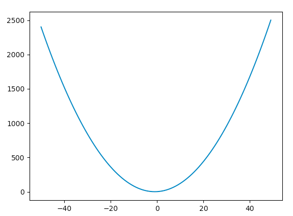
import matplotlib.pyplot as plt

a=[]
b=[]
# y=0
# x=-50

for x in range(-50,50,1):
    y=x**2+2*x+2
    a.append(x)
    b.append(y)
    #x= x+1

fig= plt.figure()
axes=fig.add_subplot(111)
axes.plot(a,b)
plt.show()
Hence, It is secured that SGD guides us to global optimum.
Then, with regard to the updating rule, it is particularly simple.
Pseudo code: Update = step-size x prediction error x feature value.
\nabla_w \hat{v}(S, w) = x(S)\\
\Delta w = \alpha (v_π (S) - \hat{v}(S, w))x(S)
In fact, in above math equations, $x$ indicates the data. However, it includes unusual formatted data. That is called "one-hot" format.
x(S) = \Biggl(
\begin{matrix}
1(S = s_1)\\
\vdots\\
1(S = s_n)
\end{matrix}
\Biggl)\\
example(if \space S = s_1) => \Biggl(
\begin{matrix}
1\\
0\\
\vdots\\
0
\end{matrix}
\Biggl)\\
\hat{v}(S, w) = \Biggl(
\begin{matrix}
1(S = s_1)\\
\vdots\\
1(S = s_n)
\end{matrix}
\Biggl)

\Biggl(
\begin{matrix}
w_1\\
\vdots\\
w_n
\end{matrix}\Biggl)
Incremental Prediction algorithms
Finally we have come to the adaptation step of seen methods(approximation of function with SGD updating).
- For MC, the target is the return $G_t$.
\Delta w = \alpha(G_t - \hat{v}(S_t, w))\nabla_w \hat{v}(S_t, w)\\
= \alpha(G_t - \hat{v}(S_t, w))\nabla_w x(S_t)
- For TD(0), the target is the TD target: $R_{t+1} + \gamma \hat{v}(S_{t+1}, w)$
\Delta w = \alpha(R_{t+1} + \gamma \hat{v}(S_{t+1}, w) - \hat{v}(S_t, w))\nabla_w \hat{v}(S_t, w)\\
= \alpha \delta x(S)
- For TD($\lambda$), the target is the $\lambda$-return $G^{\lambda}_t$
- Forward view
\Delta w = \alpha( G^{\lambda}_t - \hat{v}(S_t, w)) \nabla_w \hat{v}(S_t, w)\\
= \alpha( G^{\lambda}_t - \hat{v}(S_t, w)) \nabla_w x(S_t)
- Backward view
\delta_t = R_{t+1} + \gamma \hat{v}(S_{t+1}, w) - \hat{v}(S_t, w)\\
E_t = \gamma \lambda E_{t-1} + x(S_t)\\
\Delta w = \alpha \delta_t E_t
Incremental Control Algorithm
With the knowledge of prediction algorithms, we can move on to approximation of action-value function.
First of all, let us define the action-value function approximation.
$ \hat{q}(S, A, w) \approx q_π(S, A)$
Then, to optimise this estimate, we define the cost function using MSE.
$J(w) = E_π[(q_π(S,A) - \hat{q}(S, A, w))^2]$
And applying SGD method, we can find a local minimum.
-\frac{1}{2}\nabla_w J(w) = (q_π(S, A) - \hat{q}(S, A, w))\nabla_w \hat{q}(S, A, w)\\
\Delta w = \alpha (q_π(S, A) - \hat{q}(S, A, w))\nabla_w \hat{q}(S, A, w)
To play with this theory, we should clarify the input data. The format of input data is described below.
x(S, A) = \Biggl(
\begin{matrix}
x_1(S , A)\\
\vdots\\
x_n(S, A)
\end{matrix}
\Biggl)\\
With these defined prerequisites, we can represent an action-value function by linear combination of features.
$ \hat{q}(S, A, w) = x(S, A)^Tw = \sum^n_{j=1}x_j(S, A)w_j $
Hence, SGD update method will look like below.
\nabla_w \hat{q}(S, A, w) = x(S, A)\\
\Delta w = \alpha(q_π(S, A) - \hat{q}(S, A, w))x(S, A)
Let's see how does each algorithm look based on above equations.
- For MC, the target is the return $G_t$.
\Delta w = \alpha(G_t - \hat{q}(S_t, A, w))\nabla_w \hat{q}(S_t, A, w)\\
= \alpha(G_t - \hat{q}(S_t, A, w))\nabla_w x(S_t, A)
- For TD(0), the target is the TD target: $R_{t+1} + \gamma \hat{v}(S_{t+1}, w)$
\Delta w = \alpha(R_{t+1} + \gamma \hat{q}(S_{t+1}, A, w) - \hat{q}(S_t, A, w))\nabla_w \hat{q}(S_t, A, w)\\
= \alpha \delta x(S_t, A)
- For TD($\lambda$), the target is the $\lambda$-return $G^{\lambda}_t$
- Forward view
\Delta w = \alpha( G^{\lambda}_t - \hat{q}(S_t, A, w)) \nabla_w \hat{q}(S_t, A, w)\\
= \alpha( G^{\lambda}_t - \hat{q}(S_t, A, w)) \nabla_w x(S_t, A)
- Backward view
\delta_t = R_{t+1} + \gamma \hat{q}(S_{t+1}, A, w) - \hat{q}(S_t, A, w)\\
E_t = \gamma \lambda E_{t-1} + x(S_t, A)\\
\Delta w = \alpha \delta_t E_t
Since it is a bit beyond the scope of this article, we would like to skip for now. But indeed, there are some variants other than above.
Gradient TD learning: https://arxiv.org/pdf/1611.09328.pdf
Gradient Q-learning: https://arxiv.org/pdf/1611.01626.pdf
Batch Reinforcement Learning
In this section, we are going to learn RL for Batched datasets.
The word "batch" is quite common in machine learning domain nowadays, but what exactly mean in RL domain?
So firstly, let us touch a point on the difference between online and batch RL.
On-line RL: integrates data collection and optimization
- Select actions in environment and at the same time update parameters based on each observed $(s,a,s’,r)$
Batch RL: decouples data collection and optimization - First generate/collect experience in the environment giving a data set of state-action-reward-state pairs {$(s_i,a_i,r_i,s_i’)$}
- Bear in mind that Batch algorithms ignore the exploration-exploitation problem, and do their best with the data they have.
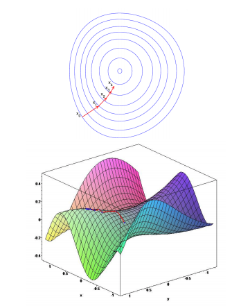
Example of batch RL from Alan Fern's slides
So let's dig in more!
Least Squares Prediction
Firstly, let's figure out the appearance of basic requirements.
Value function approximation: $\hat{v}(S, w) \approx v_π(S)$
Experience D:
D = \big((s_1, v^π_1), (s_2, v^π_2) ... (s_T, v^π_T)\big)
Least Squared optimisation: finding parameter vector w minimising sum-squared error between the estimate and the target.
LS(s) = \sum^T_{t=1}(v^π_t - \hat{v}(s_t, w))^2\\
= E_D[(v^π - \hat{v}(s, w))^2]
We would like to combine the concept of SGD and LS in RL.
And actually if you look at some relatively new research papers, they are frequently using the word "Experience Replay". But what is it?
Experience Replay: This means instead of running Q-learning on state/action pairs as they occur during simulation or actual experience, the system stores the data discovered for [state, action, reward, next_state] - typically in a large table. Note this does not store associated values - this is the raw data to feed into action-value calculations later.
This explanation is inspired by Neil Slater
By now, we have got enough of basic prerequisites. So let's jump into more fancy RL world.
SGD with Experience Replay
Logic
Given experience consisting of paris, we could define the dataset as below.
D = \big( (s_1, v^π_1), (s_2, v^π_2) ... (s_T, v^π_T) \big)
Repeat DO
- sample state, value from experience: $(s, v^π) \sim D$
- apply SGD update: $\Delta w = \alpha(v^π - \hat{v}(S, w))\nabla_w \hat{v}(S, w)$
- converges to LS solution: $w^π = argmin_w LS(w)$
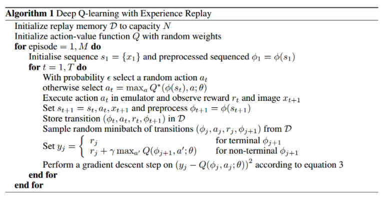
Deep Q-Network
It is approximating a q-function by deep convolutional neural network and using variant of stochastic gradient descent update it can optimise the approximation of q-function.
So based on experience replay and computing q-learning targets, we would get the loss function below.
L_i(w_i) = E_{s,a,r,s'}[(r + \gamma max_{a'}Q(s', a',; w_i^-) - Q(s, a; w_i))^2]
Then, we can use SGD to update the weights.
Least Squares Prediction
As you can see, experience replay requires huge computational power, then it may take many iterations before convergence. Using linear value function approximation, it could converge to the optimal faster than that one.
$\hat{v}(s,w) = x(s)^Tw$
At minimum of LS(w), the expected update must be zero.
E_D[\Delta w] = 0\\
\alpha \sum^T_{t=1} x(s_t)(v^π_t - x(s_t)^Tw) = 0\\
\sum^T{t=1}x(s_t)v^π_t = \sum^T_{t=1}x(s_t)x(s_t)^Tw\\
w = \biggl( \sum^T_{t=1}x(s_t)x(s_t)^T \biggl)^{-1} \sum^T_{t=1}x(s_t)v_t^π
Least squares Control
Conventionally, in prediction problem we seek the optimal state-action value, on the other hand, in control problem we want to find the optimal action-value function.