Introduction
Gradient descent optimisation algorithms, while increasingly popular, are often used as black-box optimizers, especially when it comes to the actual implementation using some DL libraries. Indeed, practical explanations of their strengths and weaknesses are hard to come by. This article aims to provide the reader with intuitions with regard to the behaviour of different algorithms that will allow us to put them to use.
Original Papaer : https://arxiv.org/pdf/1609.04747.pdf
Gradient Descent
It is a way to minimise an objective function $J(\theta)$ parametrised by a model's parameters $\theta \in R^d$ by updating the parameters in the opposite direction of the gradient of the objective function $\nabla_{\theta}J(\theta)$ with regard to the parameters. The learning rate $\eta$ determines the size of the steps we take to discover a minimum.
Variants
- Batch Gradient Descent
- Stochastic Gradient Descent
- Mini-Batch Gradient Descent
1. Batch Gradient Descent
Vanilla gradient descent, aka batch gradient descent, computes the gradient of the cost function w.r.t. the parameters $\theta$ for the entire training dataset at once.
\theta = \theta - \eta\nabla_{\theta}J(\theta)
Since we need to calculate the gradient for the entire dataset, it takes much time than other algorithms explained later.
And it does not apply to online learning.
for i in range(epochs):
  params_grad = evaluate_gradient(loss_func, data, params)
  params = params - learning_rate * params_grad
2. Stochastic Gradient Descent
SGD, in contrast, performs a parameter update for each training example $x^{(i)}$ and $y^{(i)}$.
\theta = \theta - \eta\nabla_{\theta}J(\theta; x^{(i)}; y^{(i)})
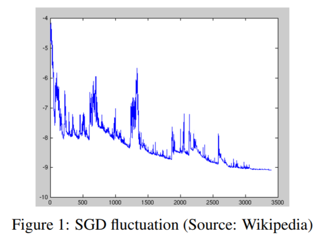
Because it computes the error/gradient and updates the parameters for each row of dataset, it can apply online learning as well. Yet, it too much frequently updates with a high variance causing the objective function to fluctuate heavily as shown below. On the other hand, we can say that this excessive fluctuation allows the algorithm to perform jumping to a new better local optimum.
for i in range(epochs):
  np.random.shuffle(data)
  for row in data:
    params_grad = evaluate_gradient(loss_func, row, params)
    params = params - learning_rate * params_grad
3. Mini-Batch Gradient Descent
Mini-batch GD finally takes the best of both worlds and performs an update or every mini-batch of $n$ training example.
\theta = \theta - \eta\nabla_{\theta}J(\theta; x^{(i:i+n)}; y^{(i:i+n)})
This benefits as shown below.
It...
1. Reduces the variance of the parameter updates
2. Can make use of highly optimised matrix optimisations common to state-of-the-art deep learning libraries efficiently. Empirically resulting, common mini-batch sizes range between 50 and 256.
for i in range(epochs):
  np.random.shuffle(data)
  for batch in get_batches(data, batch_size=50):
    params_grad = evaluate_gradient(loss_func, batch, params)
    params = params - learning_rate * params_grad
Challenges
- choosing a proper learning rate is hard.
- learning rate schedules try to adjust the learning rate during training.
- the same learning rate applies to all parameter updates.
In the following, we will outline some algorithms that are widely used by the deep learning community to deal with the aforementioned challenges.
Advanced Techniques
- Momentum Gradient Descent
- Nesterov accelerated Gradient
- Adagrad
- Adadelta
- RMSProp
- Adam
- AdaMax
- Nadam
1. Momentum Gradient Descent
Even SGD has trouble navigating ravines, such as areas where the surface curves much more steeply in one dimension than in another, which are common around local optima.
So SGD can only make hesitant minor progress along the bottom towards the local optima.
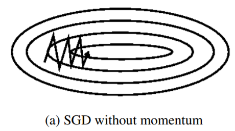
In contrast, Momentum is a method that helps accelerate SGD in the relevant direction and dampens oscillations as can b seen below.
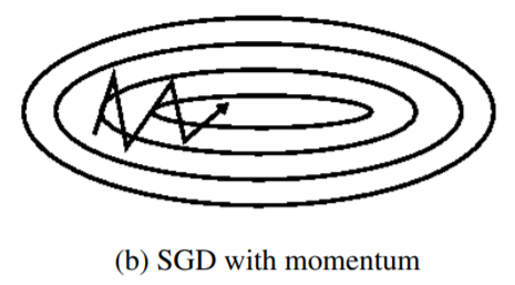
v_t = \gamma v_{t-1} + \eta\nabla+{\theta}J(\theta)\\
\theta = \theta - v_t
where momentum term : $\gamma$ is usually set to 0.9 or so.
Essentially, we can consider momentum as an accelerated speed. For instance, when we push a ball down a hill, it accumulates momentum as it rolls downhill in this case, becoming faster and faster on the way(until it reaches its terminal velocity.) So the same effect applies to our parameters updates. As a result, we gain faster convergence and reduced oscillation.
2. Nesterov accelerated Gradient
NAG(Nesterov accelerated Gradient) gives us a smarter updates method. which is aware of the direction where it is going towards. Hence it is able to slow down before the hill slopes up again.
v_t = \gamma v_{t-1} + \eta\nabla+{\theta}J(\theta - \gamma v_{t-1})\\
\theta = \theta - v_t
Computing $\theta - \gamma v_{t-1}$