前回はThe Cancer Genome Atlas(TCGA)からRNA-seqの発現量データを一括ダウンロードする方法を紹介しました。
今回はその続きとして、ダウンロードしたRNA-seqの発現量データに各サンプルが腫瘍サンプルか否かの区分情報を付与して、DESeq2での発現量比較を行います。
具体的には、腫瘍サンプル群のほうが正常サンプル群よりも有意に多く発現している遺伝子群を特定します。
<目次>
- DESeq2のインストール
- カウントデータとサンプル区分ラベルをDESeq2入力用に整形
- DESeq2の実行
1. DESeq2のインストール
DESeq2の公式サイトを参考にDESeq2をRにインストールします。
# Bioconductorパッケージマネージャーがインストールされていなければ、インストールする。
if (!requireNamespace("BiocManager", quietly = TRUE))
    install.packages("BiocManager")

# DESeq2のインストール
BiocManager::install("DESeq2")
2. カウントデータとサンプル区分ラベルをDESeq2入力用に整形
サンプルのうち、腫瘍サンプル群のほうが正常サンプル群よりも有意に多く発現している遺伝子群を特定することを考えます。
各サンプルがTumor(腫瘍)なのかNormal(正常)なのかを判断するために、TCGAから必要なサンプル区分情報をダウンロードします。
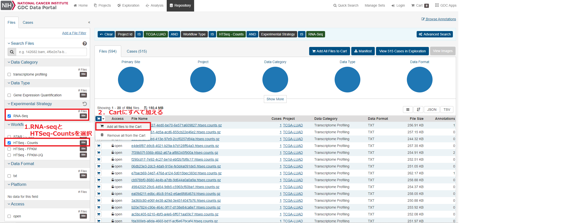
まず前回の図1から図3に従って、LUAD(=Lung Adenocarcinoma、肺腺癌)データをLUAD-TCGAから選択して、Filesに進みます。
「RNA-seq」と「HTSeq-Counts」を選択して、Cartにすべてのファイルを加えます。
Cartに移動して、中段にある「Sample Sheet」ボタンをクリックして、サンプルの区分情報をダウンロードします。その後ダウンロードしたファイルを前回のdownload_dirフォルダーにコピーします。
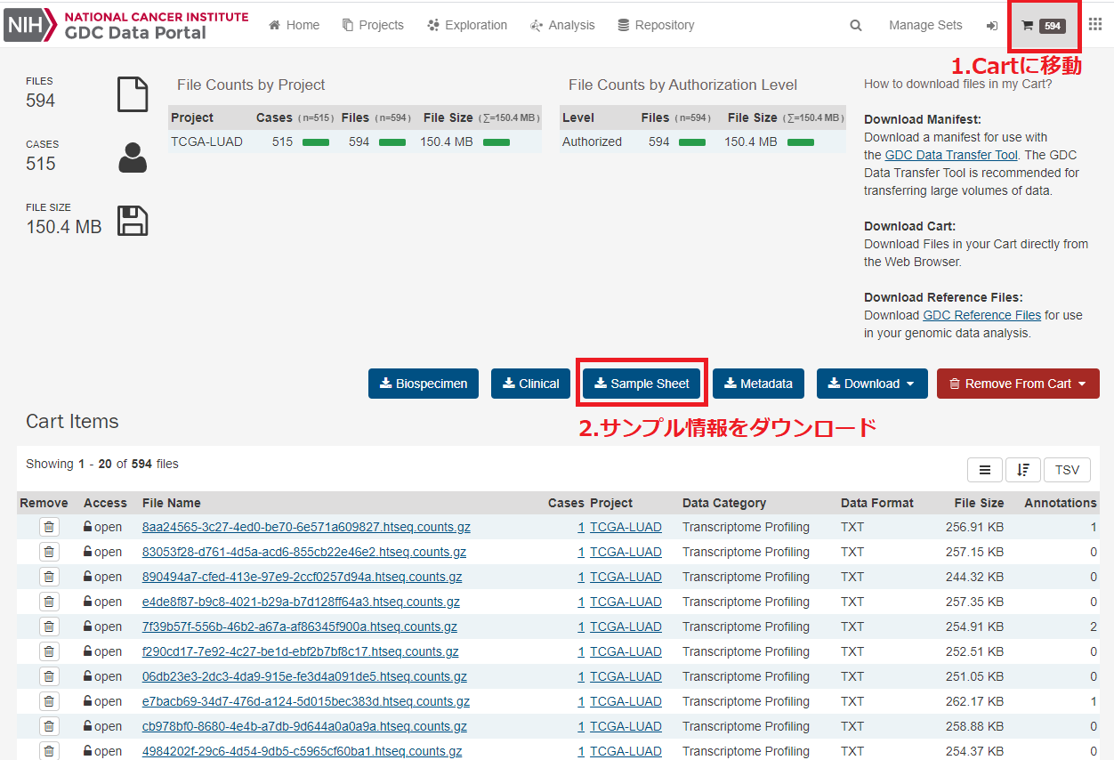
ダウンロードしたファイル(gdc_sample_sheet.2021-09-30.tsv)の中身は以下の様になっています。
File ID	File Name	Data Category	Data Type	Project ID	Case ID	Sample ID	Sample Type
6f1d55c9-b791-49a3-b664-db126f812872	8aa24565-3c27-4ed0-be70-6e571a609827.htseq.counts.gz	Transcriptome Profiling	Gene Expression Quantification	TCGA-LUAD	TCGA-J2-8194	TCGA-J2-8194-01A	Primary Tumor
5bfc07b4-30df-44eb-a05f-f85a46cfa825	83053f28-d761-4d5a-acd6-855cb22e46e2.htseq.counts.gz	Transcriptome Profiling	Gene Expression Quantification	TCGA-LUAD	TCGA-67-6215	TCGA-67-6215-01A	Primary Tumor
21f2e1df-9797-4d33-ab48-34d4b53c25d8	890494a7-cfed-413e-97e9-2ccf0257d94a.htseq.counts.gz	Transcriptome Profiling	Gene Expression Quantification	TCGA-LUAD	TCGA-91-6831	TCGA-91-6831-11A	Solid Tissue Normal
(以下省略)
このファイルのうち1列目(File ID)と2列目(File Name)を用いてファイル名の指定し、最終7列目(Sample Type)を用いて各サンプルがTumor(=Primary Tumor)かNormal(=Solid Tissue Normal)かO(その他)かを判断します。今回は簡単のため、TumorとNormalの場合のみを残して、後流の解析に用いることにします。
# !/usr/local/bin/miniconda3/bin/python
import os
import csv
import pandas as pd
import copy

cancer_type = "LUAD"
metadata_path = "gdc_sample_sheet.2021-09-30.tsv"
counter = 0
name_list = []
type_list = []
global df
with open(metadata_path, newline='') as f_metadata:
        reader = csv.reader(f_metadata, delimiter='\t')
        header = next(reader)
        for col in csv.reader(f_metadata, delimiter='\t'):
                count_file = col[0] + "/" + col[1]
                name = col[1].replace(".htseq.counts..gz", "")
                if col[7] == "Primary Tumor":
                        name_list.append(name)
                        type_list.append("Tumor")
                elif col[7] == "Solid Tissue Normal":
                        name_list.append(name)
                        type_list.append("Normal")
                else:
                        # TumorとNormal以外は今回は無視する
                        continue

                df_tmp = pd.read_table(count_file, compression='gzip', names=["gene", name], index_col=0, header=None, sep='\t')
                if counter == 0:
                        df = copy.deepcopy(df_tmp)
                else:
                        df = df.join(df_tmp)
                counter += 1

# 最後のほうの行にある行名が"__" から始まっている不要な行を削除する。
# 不要な行の直前までの行数をindexで数える。
col_list = df.index.tolist()
index = 0
for col_name in col_list:
        if col_name.startswith("__"):
                break
        index += 1

# output the merged count table
tsv_name = cancer_type + "_count_table.tsv"
df[0:index].to_csv(tsv_name, sep='\t')

# output types of labels
label_file = cancer_type + "_count_label.tsv"
with open(label_file, "w") as f_labels:
        f_labels.write("\t".join(name_list) + "\n")
        f_labels.write("\t".join(type_list) + "\n")
3. DESeq2の実行
Rを起動して以下のコマンドを実行して、DESeq2を実行します。
> library(DESeq2)

# 入力データのインポートと整形
> count <- read.table("LUAD_count_table.tsv", sep='\t', header=T,row.names="gene")
> group <- read.table("LUAD_count_label.tsv", sep='\t', header=T)
> group <- t(group)
> condition <- as.factor(group)
> columnData <- data.frame(row.names=colnames(count), condition)

# DESeq2の実行
> dds <- DESeqDataSetFromMatrix(countData = count, colData = columnData, design = ~ condition)
> dds <- DESeq(dds)
> res <- results(dds)

# 結果表示(先頭のみ)
> head(res)
log2 fold change (MLE): condition Tumor vs Normal
Wald test p-value: condition Tumor vs Normal
DataFrame with 6 rows and 6 columns
                     baseMean log2FoldChange     lfcSE      stat      pvalue        padj
                    <numeric>      <numeric> <numeric> <numeric>   <numeric>   <numeric>
ENSG00000000003.13 3071.05844       1.110464 0.1017972  10.90860 1.04862e-27 1.78910e-26
ENSG00000000005.5     6.24464       1.485880 0.4597028   3.23226 1.22815e-03 2.54223e-03
ENSG00000000419.11 1528.68957       0.253606 0.0761953   3.32837 8.73564e-04 1.85219e-03
ENSG00000000457.12  901.62702       0.440785 0.0646751   6.81537 9.40208e-12 5.02611e-11
ENSG00000000460.15  422.58421       1.736423 0.0975630  17.79796 7.32874e-71 1.03533e-68
ENSG00000000938.11 1355.70076      -2.110695 0.1360068 -15.51904 2.57882e-54 1.77529e-52
このうち、例えば補正後のP値であるpadjが0.01未満, 2群の発現量の比率を表すlog2FoldChangeが4より大きい, どちらもNAになっているものは除くという条件で絞り込めば、TumorのほうNormalよりも有意に発現量が多い遺伝子のリストを特定することが出来ます。
# padjがNAで無く、なおかつpadj<0.01
> padjSelection <- !is.na(res$padj) & res$padj < 0.01

# log2FoldChangeがNAで無く、なおかつlog2FoldChange>4
> log2FoldChangeSelection <- !is.na(res$log2FoldChange) & res$log2FoldChange > 4

# 上記の2条件ともに満たす場合
> selection <- padjSelection & log2FoldChangeSelection
> res[selection,]
log2 fold change (MLE): condition Tumor vs Normal
Wald test p-value: condition Tumor vs Normal
DataFrame with 715 rows and 6 columns
                    baseMean log2FoldChange     lfcSE      stat      pvalue        padj
                   <numeric>      <numeric> <numeric> <numeric>   <numeric>   <numeric>
ENSG00000002726.18 1847.3914        4.97759  0.299125  16.64052 3.54512e-62 3.44735e-60
ENSG00000005073.5    22.5651        4.13648  0.475638   8.69671 3.41649e-18 3.03571e-17
ENSG00000006047.11  254.8172        4.73601  0.278543  17.00282 7.82567e-65 8.59238e-63
ENSG00000006377.10   43.7775        5.01161  0.443450  11.30141 1.29125e-29 2.48896e-28
ENSG00000008197.4    57.4445        6.99077  0.585812  11.93348 7.91947e-33 1.83574e-31
...                      ...            ...       ...       ...         ...         ...
ENSG00000280081.2   15.66004        6.78013  0.783610   8.65243 5.04133e-18 4.42955e-17
ENSG00000280151.1    7.06716        4.76500  0.536065   8.88886 6.17402e-19 5.77707e-18
ENSG00000280171.1    7.55158        4.75887  0.531934   8.94636 3.67382e-19 3.47965e-18
ENSG00000281097.1   15.22247        5.12585  0.419723  12.21247 2.66665e-34 6.72008e-33
ENSG00000281566.1    5.13694        4.50152  0.979634   4.59510 4.32537e-06 1.27639e-05