このテーマを先に書く予定にしていたのですが、CNNの実装の方を先に進めてしまいました。
あらためて、データ拡張のテーマで書きたいと思います。
精度を向上される方法としてデータ拡張を考えます。
データ拡張
MNISTは、数字の画像です。手書きする場合に、左右や上下に寄ったり、傾けて書いてしまったり、大きく書く人もいれば、小さく書く人もいます。
それぞれバリエーションを増やして考えてみましょう。
上下左右に1ピクセル移動
もとの画像から上下、左右に1ピクセル移動した画像を考えます。
実際に1ピクセルずらした画像を生成してみます。プログラムは、ひとつ先になりますが、「ディープラーニングを実装から学ぶ(8)実装変更」を利用します。
データの読み込み
x_train, t_train, x_test, t_test = load_mnist('c:\\mnist\\')
data_normalizer = create_data_normalizer(min_max)
nx_train, data_normalizer_stats = train_data_normalize(data_normalizer, x_train)
nx_test                         = test_data_normalize(data_normalizer, x_test)
画像として処理するため、28 $ \times $ 28にreshapeします。
nx_train0 = nx_train.reshape(nx_train.shape[0], 28, 28)
上下、左右に1ピクセルずらします。
# 領域確保
nx_train_u1 = np.zeros_like(nx_train0)
nx_train_d1 = np.zeros_like(nx_train0)
nx_train_l1 = np.zeros_like(nx_train0)
nx_train_r1 = np.zeros_like(nx_train0)
# 1ピクセルずらす
nx_train_u1[:, 0:27, :] = nx_train0[:, 1:28, :] # 上
nx_train_d1[:, 1:28, :] = nx_train0[:, 0:27, :] # 下
nx_train_l1[:, :, 0:27] = nx_train0[:, :, 1:28] # 左
nx_train_r1[:, :, 1:28] = nx_train0[:, :, 0:27] # 右
学習データの最初のデータを表示してみましょう。
import matplotlib.pyplot as plt

plt.figure(figsize=(20, 6))
plt.subplot(1, 5, 1)
plt.imshow(nx_train0[0], 'gray')
plt.subplot(1, 5, 2)
plt.imshow(nx_train_u1[0], 'gray')
plt.subplot(1, 5, 3)
plt.imshow(nx_train_d1[0], 'gray')
plt.subplot(1, 5, 4)
plt.imshow(nx_train_l1[0], 'gray')
plt.subplot(1, 5, 5)
plt.imshow(nx_train_r1[0], 'gray')
plt.show()
左から、元画像、1ピクセル上、下、左、右に移動した画像です。
元データと結合し、学習してみましょう。
concatenateを使って、元の学習データと上下左右に移動した学習データを結合します。正解データも併せて結合します。
ニューラルネットワークで学習できるように、結合したデータを再度reshapeします。
nx_train_a = np.concatenate([nx_train0,
                             nx_train_u1, nx_train_d1, nx_train_l1, nx_train_r1])
t_train_a  = np.concatenate([t_train,
                             t_train, t_train, t_train, t_train])
nx_train_a = nx_train_a.reshape(nx_train_a.shape[0], -1)
学習です。
model = create_model(nx_train_a.shape[1]) # 28*28
model = add_layer(model, "affine1", affine, 100)
model = add_layer(model, "relu1", relu)
model = add_layer(model, "affine2", affine, 50)
model = add_layer(model, "relu2", relu)
model = add_layer(model, "affine3", affine, 10)
model = set_output(model, softmax)
model = set_error(model, cross_entropy_error)

epoch = 50
batch_size = 100
np.random.seed(10)
model, optimizer, learn_info = learn(model, nx_train_a, t_train_a, nx_test, t_test, batch_size=batch_size, epoch=epoch)
input - 0 784
affine1 affine 784 100
relu1 relu 100 100
affine2 affine 100 50
relu2 relu 50 50
affine3 affine 50 10
output softmax 10
error cross_entropy_error
0 0.08366 2.48469637584 0.0838 2.4902096706
1 0.926196666667 0.246580899532 0.9725 0.0893588543072
2 0.970636666667 0.09627760042 0.9799 0.0664156407996
3 0.97803 0.0712111672755 0.9813 0.0583722640259
・・・
47 0.999983333333 0.000606742459909 0.9862 0.0749501409849
48 0.999973333333 0.000574929201213 0.9859 0.0741143480054
49 0.999976666667 0.000539722596716 0.9854 0.0755892526723
50 0.99998 0.000518507849132 0.9859 0.0761595984635
所要時間 = 11 分 57 秒
途中は、省略しましたが、なんと、テストデータの正解率が、98.5%を超えました。
もともとこのモデルでは、97.8%程度の正解率だったのですが、大幅に精度向上しました。
斜め方向に1ピクセル移動
左上、左下、右上、右下方向に各1ピクセル移動します。
# 領域確保
nx_train_ul1 = np.zeros_like(nx_train0)
nx_train_dl1 = np.zeros_like(nx_train0)
nx_train_ur1 = np.zeros_like(nx_train0)
nx_train_dr1 = np.zeros_like(nx_train0)
# 1ピクセルずらす
nx_train_ul1[:, 0:27, 0:27] = nx_train0[:, 1:28, 1:28] # 左上
nx_train_dl1[:, 1:28, 0:27] = nx_train0[:, 0:27, 1:28] # 左下
nx_train_ur1[:, 0:27, 1:28] = nx_train0[:, 1:28, 0:27] # 右上
nx_train_dr1[:, 1:28, 1:28] = nx_train0[:, 0:27, 0:27] # 右下
移動した画像を表示します。
import matplotlib.pyplot as plt

plt.figure(figsize=(20,6))
plt.subplot(1, 5, 1)
plt.imshow(nx_train0[0], 'gray')
plt.subplot(1, 5, 2)
plt.imshow(nx_train_ul1[0], 'gray')
plt.subplot(1, 5, 3)
plt.imshow(nx_train_dl1[0], 'gray')
plt.subplot(1, 5, 4)
plt.imshow(nx_train_ur1[0], 'gray')
plt.subplot(1, 5, 5)
plt.imshow(nx_train_dr1[0], 'gray')
plt.show()

左から、元画像、1ピクセル左上、左下、右上、右下に移動した画像です。
データを結合し、学習してみます。
nx_train_a = np.concatenate([nx_train0,
                             nx_train_ul1, nx_train_dl1, nx_train_ur1, nx_train_dr1])
t_train_a  = np.concatenate([t_train,
                             t_train, t_train, t_train, t_train])
nx_train_a = nx_train_a.reshape(nx_train_a.shape[0], -1)
model = create_model(nx_train_a.shape[1]) # 28*28
model = add_layer(model, "affine1", affine, 100)
model = add_layer(model, "relu1", relu)
model = add_layer(model, "affine2", affine, 50)
model = add_layer(model, "relu2", relu)
model = add_layer(model, "affine3", affine, 10)
model = set_output(model, softmax)
model = set_error(model, cross_entropy_error)

epoch = 50
batch_size = 100
np.random.seed(10)
model, optimizer, learn_info = learn(model, nx_train_a, t_train_a, nx_test, t_test, batch_size=batch_size, epoch=epoch)
input - 0 784
affine1 affine 784 100
relu1 relu 100 100
affine2 affine 100 50
relu2 relu 50 50
affine3 affine 50 10
output softmax 10
error cross_entropy_error
0 0.0852033333333 2.47946580893 0.0838 2.4902096706
1 0.919126666667 0.270817654038 0.9745 0.0892861033313
2 0.967356666667 0.108367497164 0.9798 0.0653965367596
3 0.97465 0.0833861145689 0.9801 0.0630435421457
・・・
42 0.999126666667 0.00366044850393 0.9872 0.0643891794085
・・・
48 0.999836666667 0.00131985184222 0.9869 0.0681634018706
49 0.999923333333 0.00104220397953 0.9867 0.0671451074972
50 0.999926666667 0.000921167842613 0.9866 0.069162449616
所要時間 = 12 分 2 秒
一時的ですが、テストデータの正解率が98.7%を超えました。
すごいですね。
拡大・縮小
今度は、拡大・縮小を考えてみます。
拡大、縮小は、画像の中心を基準に拡大、縮小した方が良さそうです。
画像(28 $ \times $ 28)の中心を(0,0)とします。各ピクセルを1 $ \times $ 1の正方形を考え、その中心(+0.5)が倍率を掛けたあとにどこのマトリックスに入るか考えます。倍率を掛けた値が入った場所に、元の画像のピクセルを代入します。ただし、元の画像からはみ出す場合は無視します。
以下のような、拡大・縮小を行う関数を作成しました。倍率は、例えば、1.5倍としたい場合は、0.5を、0.5倍に縮小した場合は、-0.5を指定します。
def scaling(img, factor):
    d, h, w = img.shape
    mw = int(w/2) # 横方向の中心
    mh = int(h/2) # 縦方向の中心
    # 倍率
    factor1 = 1 + factor

    img_s = np.zeros_like(img)
    for y in range(h):
        for x in range(w):
            x_s = int((x + 0.5 - mw) * factor1 + mw)
            y_s = int((y + 0.5 - mh) * factor1 + mh)
            if y_s < h and x_s < w and y_s >= 0 and x_s >= 0:
                img_s[:, y_s, x_s] = img[:, y, x]

    return img_s
中心から1ピクセル分拡大、縮小、2ピクセル分拡大、縮小した画像を作成します。
# 1/14 拡大
nx_train_s1 = scaling(nx_train0, 1/14)
# 1/14 縮小
nx_train_s_1 = scaling(nx_train0, -1/14)
# 2/14 拡大
nx_train_s2 = scaling(nx_train0, 2/14)
# 2/14 縮小
nx_train_s_2 = scaling(nx_train0, -2/14)
画像を表示してみましょう。
import matplotlib.pyplot as plt

plt.figure(figsize=(20,6))
plt.subplot(1, 5, 1)
plt.imshow(nx_train0[0], 'gray')
plt.subplot(1, 5, 2)
plt.imshow(nx_train_s1[0], 'gray')
plt.subplot(1, 5, 3)
plt.imshow(nx_train_s_1[0], 'gray')
plt.subplot(1, 5, 4)
plt.imshow(nx_train_s2[0], 'gray')
plt.subplot(1, 5, 5)
plt.imshow(nx_train_s_2[0], 'gray')
plt.show()

左から元画像、1/14拡大、1/14縮小、2/14拡大、2/14縮小した画像です。拡大した画像は、一部色が抜け落ちています。単純にピクセル単位で拡大したためです。本来であれば、間を埋めるべきでしょうが、ここでは簡単のためこのままとします。
学習してみましょう。
nx_train_a = np.concatenate([nx_train0,
                             nx_train_s1, nx_train_s_1, nx_train_s2, nx_train_s_2])
t_train_a  = np.concatenate([t_train,
                             t_train, t_train, t_train, t_train])
nx_train_a = nx_train_a.reshape(nx_train_a.shape[0], -1)
model = create_model(nx_train_a.shape[1]) # 28*28
model = add_layer(model, "affine1", affine, 100)
model = add_layer(model, "relu1", relu)
model = add_layer(model, "affine2", affine, 50)
model = add_layer(model, "relu2", relu)
model = add_layer(model, "affine3", affine, 10)
model = set_output(model, softmax)
model = set_error(model, cross_entropy_error)

epoch = 50
batch_size = 100
np.random.seed(10)
model, optimizer, learn_info = learn(model, nx_train_a, t_train_a, nx_test, t_test, batch_size=batch_size, epoch=epoch)
input - 0 784
affine1 affine 784 100
relu1 relu 100 100
affine2 affine 100 50
relu2 relu 50 50
affine3 affine 50 10
output softmax 10
error cross_entropy_error
0 0.0855266666667 2.46674428198 0.0838 2.4902096706
1 0.92825 0.240204755982 0.9655 0.108575114375
2 0.97106 0.0963900778403 0.9736 0.0827436491121
3 0.97861 0.0690451169498 0.9774 0.0737244204491
・・・
48 1.0 0.000330579877744 0.9849 0.0900380783926
49 1.0 0.000315429347481 0.985 0.0901784863912
50 1.0 0.000308258152137 0.9853 0.0900276969017
所要時間 = 12 分 21 秒
こんな画像でも、テストデータの正解率が98.5%を超えました。
回転
今度は、画像を回転してみましょう。
回転は、以下で計算できるようです。
x_r = x \cos\theta - y \sin\theta\\
y_r = x \sin\theta + y \cos\theta
回転の関数を作成します。基本的に、拡大、縮小の関数と同じですが、回転後の座標計算に上の計算式を用います。
回転は、角度で指定しますが、内部的にはラジアンに変換しています。
def rotation(img, angle):
    d, h, w = img.shape
    mw = int(w/2) # 横方向の中心
    mh = int(h/2) # 縦方向の中心
    # 度→ラジアン
    rd = np.radians(angle)

    img_r = np.zeros_like(img)
    for y in range(h):
        for x in range(w):
            x_r = int((x + 0.5 - mw) * np.cos(rd) - (y + 0.5 - mh) * np.sin(rd) + mw)
            y_r = int((x + 0.5 - mw) * np.sin(rd) + (y + 0.5 - mh) * np.cos(rd) + mh)
            if y_r < h and x_r < w and y_r >= 0 and x_r >= 0:
                img_r[:, y_r, x_r] = img[:, y, x]

    return img_r
5度と10度、右回転、左回転してみます。
# 右5度
nx_train_rr5 = rotation(nx_train0, 5)
# 左5度
nx_train_rl5 = rotation(nx_train0, -5)
# 右10度
nx_train_rr10 = rotation(nx_train0, 10)
# 左10度
nx_train_rl10 = rotation(nx_train0, -10)
回転した画像を表示してみます。
import matplotlib.pyplot as plt

plt.figure(figsize=(20,6))
plt.subplot(1, 5, 1)
plt.imshow(nx_train0[0], 'gray')
plt.subplot(1, 5, 2)
plt.imshow(nx_train_rr5[0], 'gray')
plt.subplot(1, 5, 3)
plt.imshow(nx_train_rl5[0], 'gray')
plt.subplot(1, 5, 4)
plt.imshow(nx_train_rr10[0], 'gray')
plt.subplot(1, 5, 5)
plt.imshow(nx_train_rl10[0], 'gray')
plt.show()
左から、元画像、5度右回転、5度左回転、10度右回転、10度左回転です。
学習してみます。
nx_train_a = np.concatenate([nx_train0,
                             nx_train_rr5, nx_train_rl5, nx_train_rr10, nx_train_rl10])
t_train_a  = np.concatenate([t_train,
                             t_train, t_train, t_train, t_train])
nx_train_a = nx_train_a.reshape(nx_train_a.shape[0], -1)
model = create_model(nx_train_a.shape[1]) # 28*28
model = add_layer(model, "affine1", affine, 100)
model = add_layer(model, "relu1", relu)
model = add_layer(model, "affine2", affine, 50)
model = add_layer(model, "relu2", relu)
model = add_layer(model, "affine3", affine, 10)
model = set_output(model, softmax)
model = set_error(model, cross_entropy_error)

epoch = 50
batch_size = 100
np.random.seed(10)
model, optimizer, learn_info = learn(model, nx_train_a, t_train_a, nx_test, t_test, batch_size=batch_size, epoch=epoch)
input - 0 784
affine1 affine 784 100
relu1 relu 100 100
affine2 affine 100 50
relu2 relu 50 50
affine3 affine 50 10
output softmax 10
error cross_entropy_error
0 0.0820433333333 2.48167021584 0.0838 2.4902096706
1 0.931516666667 0.226611783988 0.9621 0.113782217537
2 0.9719 0.0922384981901 0.976 0.0748703944606
3 0.979336666667 0.066925936365 0.9781 0.068018436347
・・・
48 1.0 0.00029141952688 0.9832 0.10293328727
49 1.0 0.000279634404026 0.9836 0.103241994354
50 1.0 0.000271669149904 0.9835 0.10361414012
所要時間 = 12 分 30 秒
今までより精度は悪いようですが、それでもテストデータの正解率が、98.3%になりました。
参考
比較のためデータを5倍して試してみました。
nx_train_a = np.concatenate([nx_train0,
                             nx_train0, nx_train0, nx_train0, nx_train0])
t_train_a  = np.concatenate([t_train,
                             t_train, t_train, t_train, t_train])
nx_train_a = nx_train_a.reshape(nx_train_a.shape[0], -1)
model = create_model(nx_train_a.shape[1]) # 28*28
model = add_layer(model, "affine1", affine, 100)
model = add_layer(model, "relu1", relu)
model = add_layer(model, "affine2", affine, 50)
model = add_layer(model, "relu2", relu)
model = add_layer(model, "affine3", affine, 10)
model = set_output(model, softmax)
model = set_error(model, cross_entropy_error)

epoch = 50
batch_size = 100
np.random.seed(10)
model, optimizer, learn_info = learn(model, nx_train_a, t_train_a, nx_test, t_test, batch_size=batch_size, epoch=epoch)
input - 0 784
affine1 affine 784 100
relu1 relu 100 100
affine2 affine 100 50
relu2 relu 50 50
affine3 affine 50 10
output softmax 10
error cross_entropy_error
0 0.0813333333333 2.48924898315 0.0838 2.4902096706
1 0.9435 0.191556512324 0.9651 0.111288472427
2 0.981486666667 0.0622536601435 0.9756 0.0810758990201
3 0.990093333333 0.0344365112931 0.979 0.0723178153291
・・・
48 1.0 0.000107176488713 0.9805 0.110250079283
49 1.0 0.000104167740987 0.9804 0.110940048671
50 1.0 0.000101417755015 0.9808 0.11114425684
所要時間 = 10 分 45 秒
若干、性能が向上しました。
今までの結果を表にまとめます。
テストデータの50エポック学習後の正解率と50エポック中の最大の正解率です。
| データ拡張方法 | テスト正解率 | テスト最大 |
|---|---|---|
| 上下左右に1ピクセル移動 | 98.59 | 98.62 |
| 斜め方向に1ピクセル移動 | 98.66 | 98.72 |
| 拡大・縮小(1/14,2/14拡大・縮小) | 98.53 | 98.56 |
| 回転(5度、10度、右左回転) | 98.35 | 98.37 |
| 参考(データ5倍) | 98.08 | 98.11 |
他にも、反転が考えられますが、MNISTは数字のため、反転すると別物になってしまいます。
データ生成
このようにデータを増やしていけば精度があがるかもしれませんが、学習に大量のメモリと時間が必要となります。別のアプローチを考えます。
乱数によるデータ生成
画像に対して、移動、回転、拡大・縮小を行った画像を生成します。どれだけ移動するかは毎回乱数によって決定します。
まず、画像の移動、回転、拡大・縮小を考えます。
以下の式で表せます。
x_{gen} = (x\cos\theta - y\sin\theta) * f_x + d_x\\
y_{gen} = (x\sin\theta + y\cos\theta) * f_y + d_y
$ d_x $ : 横方向の移動
$ d_y $ : 縦方向の移動
$ f_x $ : 横方向の拡大・縮小
$ f_y $ : 縦方向の拡大・縮小
$ \theta $ : 回転角度
これらの値を乱数で決める関数です。
scaling関数やrotation関数を参考に、以下のように作成しました。
移動距離、拡大・縮小率、回転角度は、指定されたパラメータ範囲で乱数で決定します。
def generator(img, distance=0, factor=0, angle=0):
    d, h, w = img.shape
    mw = int(w/2) # 横方向の中心
    mh = int(h/2) # 縦方向の中心

    # 乱数
    distance_xr = np.random.rand() * distance*2 - distance  # 横方向の移動距離
    distance_yr = np.random.rand() * distance*2 - distance  # 縦方向の移動距離
    factor_xr = 1 + np.random.rand() * factor*2 - factor    # 横方向の拡大・縮小率
    factor_yr = 1 + np.random.rand() * factor*2 - factor    # 縦方向の拡大・縮小率
    angle_r = np.random.rand() * angle*2 - angle            # 回転角度
    # 度→ラジアン
    rd_r = np.radians(angle_r)

    # データ生成
    img_gen = np.zeros_like(img)
    for y in range(h):
        for x in range(w):
            x_gen = np.floor(((x + 0.5 - mw) * np.cos(rd_r) - (y + 0.5 - mh) * np.sin(rd_r)) * factor_xr + mw + distance_xr).astype(np.int)
            y_gen = np.floor(((x + 0.5 - mw) * np.sin(rd_r) + (y + 0.5 - mh) * np.cos(rd_r)) * factor_yr + mh + distance_yr).astype(np.int)
            # はみ出した部分は無視
            if y_gen < h and x_gen < w and y_gen >= 0 and x_gen >= 0:
                img_gen[:, y_gen, x_gen] = img[:, y, x]

    return img_gen
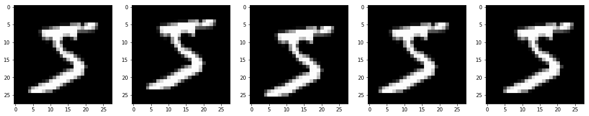
学習データの最初のデータで確認してみます。
import matplotlib.pyplot as plt

for distance, factor, angle in [[1, 1/14, 5], [2, 2/14, 10], [3, 3/14, 15]]:
    plt.figure(figsize=(20,6))
    np.random.seed(10)

    for i in range(10):
        plt.subplot(1, 10, i+1)
        plt.imshow(generator(nx_train0[0:1], distance=distance, factor=factor, angle=angle)[0], 'gray')

    plt.show()
distance=1, factor=1/14, angle=5

distance=2, factor=2/14, angle=10

distance=3, factor=3/14, angle=15

どうですか?なかなか趣がありますね。
これでもよいのですが、もう少しひねってみます。
回転で利用するsin,cosの値も乱数で別々の値とします。
def generator(img, distance=0, factor=0, angle=0):
    d, h, w = img.shape
    mw = int(w/2) # 横方向の中心
    mh = int(h/2) # 縦方向の中心

    # 乱数
    distance_xr = np.random.rand() * distance*2 - distance  # 横方向の移動距離
    distance_yr = np.random.rand() * distance*2 - distance  # 縦方向の移動距離
    factor_xr = 1 + np.random.rand() * factor*2 - factor    # 横方向の拡大・縮小率
    factor_yr = 1 + np.random.rand() * factor*2 - factor    # 縦方向の拡大・縮小率
    angle_xxr = np.random.rand() * angle*2 - angle          # 回転角度
    angle_yxr = np.random.rand() * angle*2 - angle          # 回転角度
    angle_xyr = np.random.rand() * angle*2 - angle          # 回転角度
    angle_yyr = np.random.rand() * angle*2 - angle          # 回転角度
    # 度→ラジアン
    rd_xxr = np.radians(angle_xxr)
    rd_yxr = np.radians(angle_yxr)
    rd_xyr = np.radians(angle_xyr)
    rd_yyr = np.radians(angle_yyr)

    # データ生成
    img_gen = np.zeros_like(img)
    for y in range(h):
        for x in range(w):
            x_gen = np.floor(((x + 0.5 - mw) * np.cos(rd_xxr) - (y + 0.5 - mh) * np.sin(rd_yxr)) * factor_xr + mw + distance_xr).astype(np.int)
            y_gen = np.floor(((x + 0.5 - mw) * np.sin(rd_xyr) + (y + 0.5 - mh) * np.cos(rd_yyr)) * factor_yr + mh + distance_yr).astype(np.int)
            # はみ出した部分は無視
            if y_gen < h and x_gen < w and y_gen >= 0 and x_gen >= 0:
                img_gen[:, y_gen, x_gen] = img[:, y, x]

    return img_gen
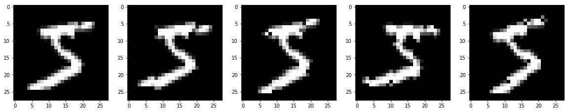
生成される画像を確認してみます。
import matplotlib.pyplot as plt

for distance, factor, angle in [[1, 1/14, 5], [2, 2/14, 10], [3, 3/14, 15]]:
    plt.figure(figsize=(20,6))
    np.random.seed(10)

    for i in range(10):
        plt.subplot(1, 10, i+1)
        plt.imshow(generator(nx_train0[0:1], distance=distance, factor=factor, angle=angle)[0], 'gray')

    plt.show()
distance=1, factor=1/14, angle=5

distance=2, factor=2/14, angle=10

distance=3, factor=3/14, angle=15

ひねりのある画像になりました。
注)
このgenerator関数は、回転角度を大きくするとまともな画像が生成されません。MNISTは、文字データのため、大きく回転しないことを前提としています。
また、拡大や回転により空白領域が生じます。物体の画像では、正式な拡大・縮小、回転関数を利用する必要があります。
学習プログラム
データを生成しながら学習できるように学習関数を変更します。
「ディープラーニングを実装から学ぶ(8)実装変更」の学習関数をベースにします。
学習関数にデータ生成関数を指定可能とします。★の部分が追加のパラメータ
# 学習関数
model, optimizer, learn_info = learn(model, x_train, t_train, x_test=None, t_test=None, batch_size=100, epoch=50, init_model_flag=True,
          optimizer=None, init_optimizer_flag=True, shuffle_flag=True, learn_info=None, generator=None, generator_param={})
# 引数
#  model  : モデル
#  x_train : 学習データ
#  t_train : 学習データ正解
#  x_test  : テストデータ(省略可)
#  t_test  : テストデータ正解(省略可)
#  batch_size : バッチサイズ
#  epoch : エポック
#  init_model_flag : モデル初期化フラグ。継続して学習する場合は、Falseを設定
#  optimizer  : オプティマイザ(省略時は、SGD)
#  init_optimizer_flag : オプティマイザ初期化フラグ。継続して学習する場合は、Falseを設定
#  shuffle_flag : シャッフルフラグ
#  learn_info : 学習情報。継続して学習する場合は、前回のlearn_infoを設定
#  generator : ★データ生成関数
#  generator_param : ★データ生成関数パラメータ
# 戻り値
#  model : モデル
#  optimizer : オプティマイザ
#  learn_info : 学習情報
ミニバッチ単位で、データを生成するようにします。
データ生成関数が設定されている場合、設定された生成関数でデータを生成し、生成したデータで学習するようにします。
        for j in range(0, x_train.shape[0], batch_size):
            # データ生成
            x_train_g = x_train[idx[j:j+batch_size]]
            if generator is not None:
                x_train_g = generator(x_train_g, **generator_param)
            # propagation
            y_train[idx[j:j+batch_size]], err, us = propagation(model, x_train_g, t_train[idx[j:j+batch_size]])
学習関数全体です。
# 学習
def learn(model, x_train, t_train, x_test=None, t_test=None, batch_size=100, epoch=50, init_model_flag=True,
          optimizer=None, init_optimizer_flag=True, shuffle_flag=True, learn_info=None, generator=None, generator_param={}):
    if init_model_flag:
        model = init_model(model)
    if optimizer is None:
        optimizer = create_optimizer(SGD)
    if init_optimizer_flag:
        optimizer = init_optimizer(optimizer, model)

    # 学習情報初期化
    learn_info = epoch_hook(learn_info, epoch, 0, model, x_train, None, t_train, x_test, t_test, batch_size)

    # エポック実行
    for i in range(epoch):
        idx = np.arange(x_train.shape[0])
        if shuffle_flag:
            # データのシャッフル
            np.random.shuffle(idx)

        # 学習
        y_train = np.zeros(t_train.shape)
        for j in range(0, x_train.shape[0], batch_size):
            # データ生成
            x_train_g = x_train[idx[j:j+batch_size]]
            if generator is not None:
                x_train_g = generator(x_train_g, **generator_param)
            # propagation
            y_train[idx[j:j+batch_size]], err, us = propagation(model, x_train_g, t_train[idx[j:j+batch_size]])
            # back_propagation
            dz, dus = back_propagation(model, x_train_g, t_train[idx[j:j+batch_size]], y_train[idx[j:j+batch_size]], us)
            # update_weight
            model, optimizer = update_weight(model, dus, optimizer)

        # 学習情報設定(エポックフック)
        learn_info = epoch_hook(learn_info, epoch, i+1, model, x_train, y_train, t_train, x_test, t_test, batch_size)

    return model, optimizer, learn_info
学習時のデータのshapeは、784です。データ生成するためには、28$ \times $28に変換する必要があります。データ生成関数内で変換するようにします。変換するデータ型は、パラメータで指定します。
def generator(img, shape=None, distance=0, factor=0, angle=0):
    img_shape = img.shape
    img_r = img
    if shape is not None:
        img_r = img.reshape((img.shape[0],) + shape)
    d, h, w = img_r.shape
    mw = int(w/2) # 横方向の中心
    mh = int(h/2) # 縦方向の中心

    # 乱数
    distance_xr = np.random.rand() * distance*2 - distance  # 左右の移動距離
    distance_yr = np.random.rand() * distance*2 - distance  # 上下の移動距離
    factor_xr = 1 + np.random.rand() * factor*2 - factor    # 左右の拡大縮小率
    factor_yr = 1 + np.random.rand() * factor*2 - factor    # 上下の拡大縮小率
    angle_xxr = np.random.rand() * angle*2 - angle          # 回転角度
    angle_yxr = np.random.rand() * angle*2 - angle          # 回転角度
    angle_xyr = np.random.rand() * angle*2 - angle          # 回転角度
    angle_yyr = np.random.rand() * angle*2 - angle          # 回転角度
    # 度→ラジアン
    rd_xxr = np.radians(angle_xxr)
    rd_yxr = np.radians(angle_yxr)
    rd_xyr = np.radians(angle_xyr)
    rd_yyr = np.radians(angle_yyr)

    # データ生成
    img_gen = np.zeros_like(img_r)
    for y in range(h):
        for x in range(w):
            x_gen = np.floor(((x + 0.5 - mw) * np.cos(rd_xxr) - (y + 0.5 - mh) * np.sin(rd_yxr)) * factor_xr + mw + distance_xr).astype(np.int)
            y_gen = np.floor(((x + 0.5 - mw) * np.sin(rd_xyr) + (y + 0.5 - mh) * np.cos(rd_yyr)) * factor_yr + mh + distance_yr).astype(np.int)
            # はみ出した部分は無視
            if y_gen < h and x_gen < w and y_gen >= 0 and x_gen >= 0:
                img_gen[:, y_gen, x_gen] = img_r[:, y, x]

    return img_gen.reshape(img_shape)
学習実行
いつもの通り、中間層を100-50エポックとして100エポック学習します。
distance,factor,angleを変更しながら実行します。
# 生成パラメータ設定
shape = (28, 28)
distance = 0 # 移動距離
factor   = 0 # 拡大・縮小率
angle    = 0 # 回転率
# モデル生成
model = create_model(nx_train.shape[1]) # 28*28
model = add_layer(model, "affine1", affine, 100)
model = add_layer(model, "relu1", relu)
model = add_layer(model, "affine2", affine, 50)
model = add_layer(model, "relu2", relu)
model = add_layer(model, "affine3", affine, 10)
model = set_output(model, softmax)
model = set_error(model, cross_entropy_error)
# 学習
epoch =100
batch_size = 100
np.random.seed(10)
model, optimizer, learn_info = learn(model, nx_train, t_train, nx_test, t_test, batch_size=batch_size, epoch=epoch,
                                     generator=generator, generator_param={"shape": shape, "distance":distance, "factor":factor, "angle":angle})
学習結果
テストデータの100エポック学習後の正解率と100エポック中の最大の正解率です。
移動のみ設定。距離を変更して実行
| distance | factor | angle | テスト正解率 | テスト最大 |
|---|---|---|---|---|
| 0 | 0 | 0 | 97.99 | 98.05 |
| 1 | 0 | 0 | 98.56 | 98.74 |
| 2 | 0 | 0 | 98.59 | 98.69 |
| 3 | 0 | 0 | 98.47 | 98.72 |
拡大・縮小のみ設定。拡大・縮小率を変更して実行
| distance | factor | angle | テスト正解率 | テスト最大 |
|---|---|---|---|---|
| 0 | 0 | 0 | 97.99 | 98.05 |
| 0 | 1/14 | 0 | 97.92 | 98.15 |
| 0 | 2/14 | 0 | 98.08 | 98.33 |
| 0 | 3/14 | 0 | 98.60 | 98.60 |
回転のみ設定。回転角度を変更して実行
| distance | factor | angle | テスト正解率 | テスト最大 |
|---|---|---|---|---|
| 0 | 0 | 0 | 97.99 | 98.05 |
| 0 | 0 | 5 | 98.24 | 98.24 |
| 0 | 0 | 10 | 98.55 | 98.70 |
| 0 | 0 | 15 | 98.46 | 98.73 |
距離を1,2、拡大・縮小率を2/14,3/14、回転角度を5,10として実行してみます。
shape = (28, 28)
for distance in [1,2]:
    for factor in [2/14, 3/14]:
        for angle in [5, 10]:
            # モデル生成
            model = create_model(nx_train.shape[1]) # 28*28
            model = add_layer(model, "affine1", affine, 100)
            model = add_layer(model, "relu1", relu)
            model = add_layer(model, "affine2", affine, 50)
            model = add_layer(model, "relu2", relu)
            model = add_layer(model, "affine3", affine, 10)
            model = set_output(model, softmax)
            model = set_error(model, cross_entropy_error)
            # 学習
            epoch =100
            batch_size = 100
            np.random.seed(10)
            model, optimizer, learn_info = learn(model, nx_train, t_train, nx_test, t_test, batch_size=batch_size, epoch=epoch,
                                                 generator=generator, generator_param={"shape": shape, "distance":distance, "factor":factor, "angle":angle})
結果です。
| distance | factor | angle | テスト正解率 | テスト最大 |
|---|---|---|---|---|
| 1 | 2/14 | 5 | 98.87 | 98.95 |
| 1 | 2/14 | 10 | 99.03 | 99.03 |
| 1 | 3/14 | 5 | 99.02 | 99.15 |
| 1 | 3/14 | 10 | 99.03 | 99.03 |
| 2 | 2/14 | 5 | 98.68 | 98.94 |
| 2 | 2/14 | 10 | 98.83 | 98.98 |
| 2 | 3/14 | 5 | 98.95 | 99.12 |
| 2 | 3/14 | 10 | 99.03 | 99.09 |
なんと、一部では、テストデータの正解率が最高で99.1%を超えました。CNNに匹敵する信じられない好結果となりました。
テストデータの正解率が最高だったdistance=2,factor=3/14,angle=10の場合、100エポック後の学習データの正解率は、約97.4%でした。もう少し学習を進めればもっと良い可能性があるため、300エポックまで実行してみます。
# 生成パラメータ設定
shape = (28, 28)
distance = 2    # 移動距離
factor   = 3/14 # 拡大・縮小率
angle    = 10   # 回転率
# モデル生成
model = create_model(nx_train.shape[1]) # 28*28
model = add_layer(model, "affine1", affine, 100)
model = add_layer(model, "relu1", relu)
model = add_layer(model, "affine2", affine, 50)
model = add_layer(model, "relu2", relu)
model = add_layer(model, "affine3", affine, 10)
model = set_output(model, softmax)
model = set_error(model, cross_entropy_error)
# 学習
epoch =300
batch_size = 100
np.random.seed(10)
model, optimizer, learn_info = learn(model, nx_train, t_train, nx_test, t_test, batch_size=batch_size, epoch=epoch,
                                     generator=generator, generator_param={"shape": shape, "distance":distance, "factor":factor, "angle":angle})
input - 0 784
affine1 affine 784 100
relu1 relu 100 100
affine2 affine 100 50
relu2 relu 50 50
affine3 affine 50 10
output softmax 10
error cross_entropy_error
0 0.0813333333333 2.48924898315 0.0838 2.4902096706
1 0.681033333333 0.981945836947 0.9321 0.241290920883
2 0.84865 0.483548855845 0.9495 0.164630707487
3 0.89265 0.347302183619 0.9619 0.124001296173
・・・
74 0.970433333333 0.0946977073154 0.9905 0.0343720184667
・・・
98 0.97295 0.0840630361126 0.9909 0.0266928733098
99 0.972733333333 0.0860101970137 0.9896 0.0334277833642
100 0.9738 0.0837216612139 0.9903 0.0306458112353
101 0.974716666667 0.0817312785596 0.9911 0.0293649995956
・・・
295 0.978783333333 0.0645823356733 0.9927 0.026440649005
296 0.980316666667 0.0617649167136 0.9922 0.0247675738371
297 0.9804 0.0617255174771 0.9923 0.0232615346676
298 0.9803 0.0616248947322 0.992 0.0221646183612
299 0.979633333333 0.0631737256453 0.9917 0.0250425930995
300 0.980716666667 0.0609466584005 0.9905 0.026128604829
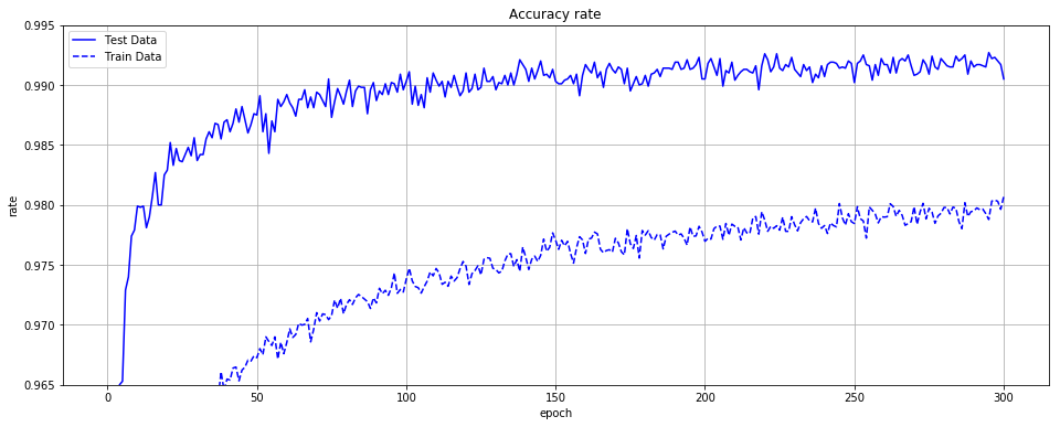
テストデータの正解率は、最高で99.27%となりました。
素晴らしい結果です。
正解率をグラフにしてみます。実線がテストデータの正解率、破線が学習データの正解率です。
import matplotlib.pyplot as plt

times = np.arange(0, epoch+1)
plt.figure(figsize=(20,8))
plt.plot(times, learn_info['accuracy_rate_test'], label="Test Data", color="blue")
plt.plot(times, learn_info['accuracy_rate_train'], label="Train Data", color="blue", linestyle="dashed")
plt.title("Accuracy rate")
plt.xlabel("epoch")
plt.ylabel("rate")
plt.ylim(0.965,0.995)
plt.legend()
plt.grid()
plt.show()
最後に、ノード数を増やして確認してみます。パラメータは、同じくdistance=2,factor=3/14,angle=10です。100エポック実行しました。
| ノード数 | テスト正解率 | テスト最大 |
|---|---|---|
| 100- 50 | 99.03 | 99.09 |
| 200-100 | 99.21 | 99.21 |
| 500-250 | 99.25 | 99.33 |
ノード数を増やすと、テストデータの正解率は、99.3%を超えました。
今回は、データ拡張に対応してみました。MNISTでは、CNNに匹敵する好成績となりました。本当にびっくりです。
プログラム全体
プログラム
import gzip
import numpy as np
# MNIST読み込み
def load_mnist( mnist_path ) :
    return _load_image(mnist_path + 'train-images-idx3-ubyte.gz'), \
           _load_label(mnist_path + 'train-labels-idx1-ubyte.gz'), \
           _load_image(mnist_path + 't10k-images-idx3-ubyte.gz'), \
           _load_label(mnist_path + 't10k-labels-idx1-ubyte.gz')
def _load_image( image_path ) :
    # 画像データの読み込み
    with gzip.open(image_path, 'rb') as f:
        buffer = f.read()
    size = np.frombuffer(buffer, np.dtype('>i4'), 1, offset=4)
    rows = np.frombuffer(buffer, np.dtype('>i4'), 1, offset=8)
    columns = np.frombuffer(buffer, np.dtype('>i4'), 1, offset=12)
    data = np.frombuffer(buffer, np.uint8, offset=16)
    image = np.reshape(data, (size[0], rows[0]*columns[0]))
    image = image.astype(np.float32)
    return image
def _load_label( label_path ) :
    # 正解データ読み込み
    with gzip.open(label_path, 'rb') as f:
        buffer = f.read()
    size = np.frombuffer(buffer, np.dtype('>i4'), 1, offset=4)
    data = np.frombuffer(buffer, np.uint8, offset=8)
    label = np.zeros((size[0], 10))
    for i in range(size[0]):
        label[i, data[i]] = 1
    return label

# 正規化関数
def min_max(x, stats, axis=None):
    if "min" not in stats:
        stats["min"] = np.min(x, axis=axis, keepdims=True) # 最小値を求める
    if "max" not in stats:
        stats["max"] = np.max(x, axis=axis, keepdims=True) # 最大値を求める
    return (x-stats["min"])/np.maximum((stats["max"]-stats["min"]),1e-7), stats

def z_score(x, stats, axis=None):
    if "mean" not in stats:
        stats["mean"] = np.mean(x, axis=axis, keepdims=True) # 平均値を求める
    if "std" not in stats:
        stats["std"]  = np.std(x, axis=axis, keepdims=True)  # 標準偏差を求める
    return (x-stats["mean"])/np.maximum(stats["std"],1e-7), stats

# affine変換
def affine(u, W, b):
    return np.dot(u, W) + b

def affine_back(dz, u, W, b, calc_du_flag=True):
    du = None
    if calc_du_flag:                        # 最初の層では、duを計算しない
        du = np.dot(dz, W.T)                # zの勾配は、今までの勾配と重みを掛けた値
    dW = np.dot(u.T, dz)                    # 重みの勾配は、zに今までの勾配を掛けた値
    db = np.dot(np.ones(u.shape[0]).T, dz)  # バイアスの勾配は、今までの勾配の値
    return du, dW, db

# 活性化関数(中間)
def sigmoid(u):
    return 1/(1 + np.exp(-u))

def sigmoid_back(dz, u, z):
    return dz * (z - z**2)

def tanh(u):
    return np.tanh(u)

def tanh_back(dz, u, z):
    return dz * (1 - z**2)
#    return dz * (1/np.cosh(u)**2)

def relu(u):
    return np.maximum(0, u)

def relu_back(dz, u, z):
    return dz * np.where(u > 0, 1, 0)

def leaky_relu(u, alpha):
    return np.maximum(u * alpha, u)

def leaky_relu_back(dz, u, z, alpha):
    return dz * np.where(u > 0, 1, alpha)

def prelu(u, alpha):
    return np.where(u > 0, u, u * alpha )

def prelu_back(dz, u, z, alpha):
    return dz * np.where(u > 0, 1, alpha), np.sum(dz * np.where(u > 0, 0, u), axis=0)/u.shape[0]

def rrelu(u, alpha):
    return np.where(u > 0, u, u * alpha )

def rrelu_back(dz, u, z, alpha):
    return dz * np.where(u > 0, 1, alpha)

def relun(u, n):
    return np.minimum(np.maximum(0, u), n)

def relun_back(dz, u, z, n):
    return dz * np.where(u > n, 0, np.where(u > 0, 1, 0))

def srelu(u, alpha):
    return np.where(u > alpha, u, alpha)

def srelu_back(dz, u, z, alpha):
    return dz * np.where(u > alpha, 1, 0)

def elu(u, alpha):
    return np.where(u > 0, u,  alpha * (np.exp(u) - 1))

def elu_back(dz, u, z, alpha):
    return dz * np.where(u > 0, 1,  alpha * np.exp(u))

def maxout(u, unit):
    u = u.reshape((u.shape[0],int(u.shape[1]/unit),unit))
    return np.max(u, axis=2)

def maxout_back(dz, u, z, unit):
    u = u.reshape((u.shape[0],int(u.shape[1]/unit),unit))
    u_max = np.argmax(u,axis=2)
    du = np.zeros_like(u)
    for i in range(du.shape[0]):
        for j in range(du.shape[1]):
            du[i,j,u_max[i,j]] = dz[i,j]
    return du.reshape((du.shape[0],int(du.shape[1]*unit)))

def identity(u):
    return u

def identity_back(dz, u, z):
    return dz

def softplus(u):
    return np.log(1+np.exp(u))

def softplus_back(dz, u, z):
    return dz * (1/(1 + np.exp(-u)))

def softsign(u):
    return u/(1+np.absolute(u))

def softsign_back(dz, u, z):
    return dz * (1/(1+np.absolute(u))**2)

def step(u):
    return np.where(u > 0, 1, 0)

def step_back(dz, u, x):
    return 0

# 活性化関数(出力)
def softmax(u):
    u = u.T
    max_u = np.max(u, axis=0)
    exp_u = np.exp(u - max_u)
    sum_exp_u = np.sum(exp_u, axis=0)
    y = exp_u/sum_exp_u
    return y.T

# 損失関数
def mean_squared_error(y, t):
    size = 1
    if y.ndim == 2:
        size = y.shape[0]
    return 0.5 * np.sum((y-t)**2)/size

def cross_entropy_error(y, t):
    size = 1
    if y.ndim == 2:
        size = y.shape[0]
    if t.shape[t.ndim-1] == 1:
        # 2値分類
        return -np.sum(t * np.log(np.maximum(y,1e-7)) + (1 - t) * np.log(np.maximum(1 - y,1e-7)))/size
    else:
        # 多クラス分類
        return -np.sum(t * np.log(np.maximum(y,1e-7)))/size

# 活性化関数(出力)+損失関数勾配
def softmax_cross_entropy_error_back(y, u, t):
    size = 1
    if y.ndim == 2:
        size = y.shape[0]
    return (y - t)/size

def sigmoid_cross_entropy_error_back(y, u, t):
    size = 1
    if y.ndim == 2:
        size = y.shape[0]
    return (y - t)/size

def identity_mean_squared_error_back(y, u, t):
    size = 1
    if y.ndim == 2:
        size = y.shape[0]
    return (y - t)/size

# 重み・バイアスの初期化
def lecun_normal(d_1, d):
    var = 1/np.sqrt(d_1)
    return np.random.normal(0, var, (d_1, d))
def lecun_uniform(d_1, d):
    min = -np.sqrt(3/d_1)
    max = np.sqrt(3/d_1)
    return np.random.uniform(min, max, (d_1, d))

def glorot_normal(d_1, d):
    var = np.sqrt(2/(d_1+d))
    return np.random.normal(0, var, (d_1, d))
def glorot_uniform(d_1, d):
    min = -np.sqrt(6/(d_1+d))
    max = np.sqrt(6/(d_1+d))
    return np.random.uniform(min, max, (d_1, d))

def he_normal(d_1, d):
    var = np.sqrt(2/d_1)
    return np.random.normal(0, var, (d_1, d))
def he_uniform(d_1, d):
    min = -np.sqrt(6/d_1)
    max = np.sqrt(6/d_1)
    return np.random.uniform(min, max, (d_1, d))

def normal_w(d_1, d, mean=0, var=1):
    return np.random.normal(mean, var, (d_1, d))
def normal_b(d, params, mean=0, var=1):
    return np.random.normal(mean, var, d)

def uniform_w(d_1, d, min=0, max=1):
    return np.random.uniform(min, max, (d_1, d))
def uniform_b(d, params, min=0, max=1):
    return np.random.uniform(min, max, d)

def zeros_w(d_1, d):
    return np.zeros((d_1, d))
def zeros_b(d):
    return np.zeros(d)

def ones_w(d_1, d):
    return np.ones((d_1, d))
def ones_b(d):
    return np.ones(d)

# 勾配法
def SGD(W, dW, lr=0.1):
    return W - lr*dW, {}

def Momentum(W, dW, lr=0.01, mu=0.9, v=None):
    if v is None: # vの初期値設定
        v = np.zeros_like(W)
    # vの更新
    v = mu * v - lr * dW
    return W + v, {"v":v}

def Nesterov(W, dW, lr=0.01, mu=0.9, v=None):
    if v is None:
        v = np.zeros_like(W)
    v = mu * v - lr * dW
    return W + v, {"v":v}

def AdaGrad(W, dW, lr=0.01, epsilon=1e-7, g=None):
    if g is None:
        g = np.zeros_like(W)
    g =  g + (dW * dW)
    return W - (lr * dW)/np.sqrt(np.maximum(g, epsilon)), {"g":g}

def RMSProp(W, dW, lr=0.001, gamma=0.9, epsilon=1e-7, g=None):
    if g is None:
        g = np.zeros_like(W)
    g =  gamma * g + (1 - gamma) * dW * dW
    return W - (lr * dW)/np.sqrt(np.maximum(g, epsilon)), {"g":g}

def Adadelta(W, dW, lr=1.0, gamma=0.9, epsilon=1e-7, g=None, s=None):
    if g is None:
        g = np.zeros_like(W)
    if s is None:
        s = np.zeros_like(W)
    g = gamma * g + (1 - gamma) * dW * dW
    newW = W - (lr * dW)/np.sqrt(np.maximum(g, epsilon)) * np.sqrt(np.maximum(s, epsilon))
    s = (1 - gamma) * (newW - W) * (newW - W) + gamma * s
    return newW, {"g":g, "s":s}

def Adam(W, dW, lr=0.001, beta1=0.9, beta2=0.999, epsilon=1e-7, k=0, m=None, v=None):
    if m is None:
        m = np.zeros_like(W)
    if v is None:
        v = np.zeros_like(W)
    k = k + 1
    m = beta1 * m + (1 - beta1) * dW
    v = beta2 * v + (1 - beta2) * dW * dW
    hatm = m / (1 - np.power(beta1, k))
    hatv = v / (1 - np.power(beta2, k))
    return W - lr / np.maximum(np.sqrt(hatv), epsilon) * hatm, {"k":k, "m":m, "v":v}

# 重み減衰
def L1_norm(W, weight_decay_lambda):
    r = np.sum(np.absolute(W))
    return r * weight_decay_lambda

def L1_norm_back(W, weight_decay_lambda):
    return np.where(W > 0, weight_decay_lambda, np.where(W < 0, -weight_decay_lambda, 0))

def L2_norm(W, weight_decay_lambda):
    r = np.sum(W**2)
    return (r * weight_decay_lambda)/2

def L2_norm_back(W, weight_decay_lambda):
    return weight_decay_lambda * W

# ドロップアウト
def dropout(z, mask):
    return z * mask

def dropout_back(dz, mask):
    return dz * mask

def set_dropout_mask(d, dropout_ratio):
    mask = np.zeros(d)
    mask = mask.flatten()
    size = mask.shape[0]
    mask_idx = np.random.choice(size, round(dropout_ratio*size), replace=False) # 通すindexの配列
    mask[mask_idx] = 1
    mask = mask.reshape(d)
    return mask

# バッチ正規化
def batch_normalization(u, gamma, beta, axis=0, u_mean=None, u_var=None):
    if u_mean is None:
        u_mean = np.mean(u, axis=axis, keepdims=True)               # 平均値を求める
    if u_var is None:
        u_var  = np.var(u, axis=axis, keepdims=True)                # 分散を求める
    u_std  = np.maximum(np.sqrt(u_var), 1e-7)                       # 標準偏差を求める
    uh = (u-u_mean)/u_std                                           # 正規化
    return gamma * uh + beta, u_mean, u_var

def batch_normalization_back(dz, u, gamma, beta, axis=0, u_mean=None, u_var=None):
    m = u.shape[axis]                                               # バッチサイズ
    if u_mean is None:
        u_mean = np.mean(u, axis=axis, keepdims=True)               # 平均値を求める
    if u_var is None:
        u_var  = np.var(u, axis=axis, keepdims=True)                # 分散を求める
    u_std  = np.maximum(np.sqrt(u_var), 1e-7)                       # 標準偏差を求める
    uh     = (u-u_mean)/u_std                                       # 正規化
    gdz    = dz * gamma
    dz_sum = np.sum(gdz * (u - u_mean), axis=axis, keepdims=True)
    dn     = (gdz - (uh * dz_sum /(m * u_std)))/ u_std
    dn_sum = np.sum(dn, axis=axis, keepdims=True)
    du     = dn - (dn_sum / m)
    if gamma.ndim == 1:
        dgamma = np.sum(uh * dz)/u.reshape(u.shape[0], -1).shape[1]
        dbeta  = np.sum(dz)/u.reshape(u.shape[0], -1).shape[1]
    else:
        dgamma = np.sum(uh * dz, axis=axis, keepdims=True)
        dbeta  = np.sum(dz, axis=axis, keepdims=True)
    return du, dgamma, dbeta, u_mean, u_var

# 正解率
def accuracy_rate(y, t):
    # 2値分類
    if t.shape[t.ndim-1] == 1:
        round_y = np.round(y)
        return np.sum(round_y == t)/y.shape[0]
    # 多クラス分類
    else:
        max_y = np.argmax(y, axis=1)
        max_t = np.argmax(t, axis=1)
        return np.sum(max_y == max_t)/y.shape[0]

# F値
def f_measure(y, t):
    TP = np.sum((y == 1) & (t==1))
    if TP == 0:
        print("TP=0")
        return 0
    FP = np.sum((y == 1) & (t==0))
    TN = np.sum((y == 0) & (t==0))
    FN = np.sum((y == 0) & (t==1))
    precision=TP/(TP+FP)
    recall = TP/(TP+FN)
    f_measure = 2*(precision*recall)/(precision+recall)
    return f_measure, precision, recall, TP, FP, TN, FN
def middle_propagation(func, u, weights, weight_decay, learn_flag, **params):
    z = func(u, **params)
    return {"u":u, "z":z}, 0

def middle_back_propagation(back_func, dz, us, weights, weight_decay, calc_du_flag, **params):
    du = back_func(dz, us["u"], us["z"], **params)
    return {"du":du}

def output_propagation(func, u, learn_flag, **params):
    z = func(u, **params)
    return {"u":u, "z":z}

# affine
def affine_init_layer(d_prev, d, weight_init_func=he_normal, weight_init_params={}, bias_init_func=zeros_b, bias_init_params={}):
    W = weight_init_func(d_prev, d, **weight_init_params)
    b = bias_init_func(d, **bias_init_params)
    return d, {"W":W, "b":b}

def affine_init_optimizer():
    sW = {}
    sb = {}
    return {"sW":sW, "sb":sb}

def affine_propagation(func, u, weights, weight_decay, learn_flag, **params):
    z = func(u, weights["W"], weights["b"])
    # 重み減衰対応
    weight_decay_r = 0
    if weight_decay is not None:
        weight_decay_r = weight_decay["func"](weights["W"], **weight_decay["params"])
    return {"u":u, "z":z}, weight_decay_r

def affine_back_propagation(back_func, dz, us, weights, weight_decay, calc_du_flag, **params):
    du, dW, db = back_func(dz, us["u"], weights["W"], weights["b"], calc_du_flag)
    # 重み減衰対応
    if weight_decay is not None:
        dW = dW + weight_decay["back_func"](weights["W"], **weight_decay["params"])
    return {"du":du, "dW":dW, "db":db}

def affine_update_weight(func, du, weights, optimizer_stats, **params):
    weights["W"], optimizer_stats["sW"] = func(weights["W"], du["dW"], **params, **optimizer_stats["sW"])
    weights["b"], optimizer_stats["sb"] = func(weights["b"], du["db"], **params, **optimizer_stats["sb"])
    return weights, optimizer_stats

# maxout
def maxout_init_layer(d_prev, d, unit=1, weight_init_func=he_normal, weight_init_params={}, bias_init_func=zeros_b, bias_init_params={}):
    W = weight_init_func(d_prev, d*unit, **weight_init_params)
    b = bias_init_func(d*unit, **bias_init_params)
    return d, {"W":W, "b":b}

def maxout_init_optimizer():
    sW = {}
    sb = {}
    return {"sW":sW, "sb":sb}

def maxout_propagation(func, u, weights, weight_decay, learn_flag, unit=1, **params):
    u_affine = affine(u, weights["W"], weights["b"])
    z   = func(u_affine, unit)
    # 重み減衰対応(未対応)
    weight_decay_r = 0
    #if weight_decay is not None:
    #    weight_decay_r = weight_decay["func"](weights["W"], **weight_decay["params"])
    return {"u":u, "z":z, "u_affine":u_affine}, weight_decay_r

def maxout_back_propagation(back_func, dz, us, weights, weight_decay, calc_du_flag, unit=1, **params):
    du_affine = back_func(dz, us["u_affine"], us["z"], unit)
    du, dW, db = affine_back(du_affine, us["u"], weights["W"], weights["b"])
    # 重み減衰対応(未対応)
    #if weight_decay is not None:
    #    dW = dW + weight_decay["back_func"](weights["W"], **weight_decay["params"])
    return {"du":du, "dW":dW, "db":db}

def maxout_update_weight(func, du, weights, optimizer_stats, **params):
    weights["W"], optimizer_stats["sW"] = func(weights["W"], du["dW"], **params, **optimizer_stats["sW"])
    weights["b"], optimizer_stats["sb"] = func(weights["b"], du["db"], **params, **optimizer_stats["sb"])
    return weights, optimizer_stats

# prelu
def prelu_init_layer(d_prev, d):
    alpha = np.zeros(d)
    return d, {"alpha":alpha}

def prelu_init_optimizer():
    salpha = {}
    return {"salpha":salpha}

def prelu_propagation(func, u, weights, weight_decay, learn_flag, **params):
    z = func(u, weights["alpha"])
    return {"u":u, "z":z}, 0

def prelu_back_propagation(back_func, dz, us, weights, weight_decay, calc_du_flag, **params):
    du, dalpha = back_func(dz, us["u"], us["z"], weights["alpha"])
    return {"du":du, "dalpha":dalpha}

def prelu_update_weight(func, du, weights, optimizer_stats, **params):
    weights["alpha"], optimizer_stats["salpha"] = func(weights["alpha"], du["dalpha"], **params, **optimizer_stats["salpha"])
    return weights, optimizer_stats

# rrelu
def rrelu_init_layer(d_prev, d, min=0.0, max=0.1):
    alpha = np.random.uniform(min, max, d)
    return d, {"alpha":alpha}

def rrelu_propagation(func, u, weights, weight_decay, learn_flag, min=0.0, max=0.1):
    z = func(u, weights["alpha"])
    return {"u":u, "z":z}, 0

def rrelu_back_propagation(back_func, dz, us, weights, weight_decay, calc_du_flag, min=0.0, max=0.1):
    du = back_func(dz, us["u"], us["z"], weights["alpha"])
    return {"du":du}

# batch_normalization
def batch_normalization_init_layer(d_prev, d, batch_norm_node=True, use_gamma_beta=True, use_train_stats=True, alpha=0.1):
    # バッチ正規化
    dim = d
    if type(d) == int:
        dim = (d,)
    # gamma,beta初期化
    if batch_norm_node:
        gamma = np.ones((1,) + dim)
        beta  = np.zeros((1,) + dim)
    else:
        gamma = np.ones(1)
        beta  = np.zeros(1)
    # 学習時の統計情報初期化
    train_mean = None
    train_var  = None
    if use_train_stats:
        if batch_norm_node:
            train_mean = np.zeros((1,) + dim)
            train_var  = np.ones((1,) + dim)
        else:
            train_mean = np.zeros(1)
            train_var  = np.ones(1)

    return d, {"gamma":gamma, "beta":beta, "use_gamma_beta":use_gamma_beta,
               "use_train_stats":use_train_stats, "alpha":alpha, "train_mean":train_mean, "train_var":train_var}

def batch_normalization_init_optimizer():
    sgamma = {}
    sbeta = {}
    return {"sgamma":sgamma, "sbeta":sbeta}

def batch_normalization_propagation(func, u, weights, weight_decay, learn_flag, **params):
    if learn_flag or not weights["use_train_stats"]:
        z, u_mean, u_var = func(u, weights["gamma"], weights["beta"])
    else:
        z, u_mean, u_var = func(u, weights["gamma"], weights["beta"], u_mean=weights["train_mean"], u_var=weights["train_var"])
    return {"u":u, "z":z, "u_mean":u_mean, "u_var":u_var}, 0

def batch_normalization_back_propagation(back_func, dz, us, weights, weight_decay, calc_du_flag, **params):
    du, dgamma, dbeta, u_mean, u_var = back_func(dz, us["u"], weights["gamma"], weights["beta"], u_mean=us["u_mean"], u_var=us["u_var"])
    return {"du":du, "dgamma":dgamma, "dbeta":dbeta, "u_mean":u_mean, "u_var":u_var}

def batch_normalization_update_weight(func, du, weights, optimizer_stats, **params):
    if weights["use_gamma_beta"]:
        weights["gamma"], optimizer_stats["sgamma"] = func(weights["gamma"], du["dgamma"], **params, **optimizer_stats["sgamma"])
        weights["beta"],  optimizer_stats["sbeta"]  = func(weights["beta"] , du["dbeta"],  **params, **optimizer_stats["sbeta"])
    if weights["use_train_stats"]:
        weights["train_mean"] = (1 - weights["alpha"]) * weights["train_mean"] + weights["alpha"] * du["u_mean"]
        weights["train_var"]  = (1 - weights["alpha"]) * weights["train_var"]  + weights["alpha"] * du["u_var"]
    return weights, optimizer_stats

# dropout
def dropout_propagation(func, u, weights, weight_decay, learn_flag, dropout_ratio=0.9):
    dropout_mask = None
    if learn_flag:
        dropout_mask = set_dropout_mask(u[-1].shape, dropout_ratio)
        z = func(u, dropout_mask)
    else:
        z = u * dropout_ratio
    return {"u":u, "z":z, "dropout_mask":dropout_mask}, 0

def dropout_back_propagation(back_func, dz, us, weights, weight_decay, calc_du_flag, dropout_ratio=0.9):
    du = back_func(dz, us["dropout_mask"])
    return {"du":du}
from collections import OrderedDict
import pickle

def create_model(d):
    # modelの生成
    model = {}
    model["input"] = {"d":d}
    model["layer"] = OrderedDict()
    model["weight_decay"] = None
    return model

def add_layer(model, name, func, d=None, **kwargs):
    # layerの設定
    model["layer"][name] = {"func":func, "back_func":eval(func.__name__ + "_back"), "d":d, "params":kwargs, "weights":None}
    return model

def set_output(model, func, **kwargs):
    # layerの設定
    model["output"] = {"func":func, "d":1, "params":kwargs}
    return model

def set_error(model, func, **kwargs):
    # layerの設定
    model["error"] = {"func":func, "d":1, "params":kwargs}
    return model

def set_weight_decay(model, func, **kwargs):
    model["weight_decay"] = {"func":func, "back_func":eval(func.__name__ + "_back"), "params":kwargs}
    return model

def init_model(model):
    # modelの初期化
    # input
    d_prev = 0
    d_next = model["input"]["d"]
    print("input", "-", d_prev, d_next)
    # layer
    d_prev = d_next
    # du計算フラグ
    calc_du_flag = False
    for k, v in model["layer"].items():
        # du計算フラグ設定
        v["calc_du_flag"] = calc_du_flag
        # 要素数取得
        d = v["d"] if v["d"] != None else d_prev
        # 重み、バイアスの初期化
        d_next = d
        if v["func"].__name__ + "_init_layer" in globals():
            init_layer_func = eval(v["func"].__name__ + "_init_layer")
            d_next, v["weights"] = init_layer_func(d_prev, d, **v["params"])
            # 以降du計算
            calc_du_flag = True
        # 要素数設定
        v["d_prev"], v["d_next"] = d_prev, d_next
        # モデル表示
        print(k, v["func"].__name__, d_prev, d_next)
        d_prev = d_next
    # output
    model["output"]["d_prev"] = d_prev
    print("output", model["output"]["func"].__name__, d_prev)
    # error
    print("error", model["error"]["func"].__name__)

    return model

def save_model(model, file_path):
    f = open(file_path, "wb")
    pickle.dump(model, f)
    f.close
    return

def load_model(file_path):
    f = open(file_path, "rb")
    model = pickle.load(f)
    f.close
    return model

def create_optimizer(func, **kwargs):
    optimizer = {"func":func, "params":kwargs}
    return optimizer

def init_optimizer(optimizer, model):
    optimizer_stats = {}
    for k, v in model["layer"].items():
        # オプティマイザの初期化
        if v["func"].__name__ + "_init_optimizer" in globals():
            init_optimizer_func = eval(v["func"].__name__ + "_init_optimizer")
            optimizer_stats[k] = init_optimizer_func()
    optimizer["stats"] = optimizer_stats

    return optimizer

def save_optimizer(optimizer, file_path):
    f = open(file_path, "wb")
    pickle.dump(optimizer, f)
    f.close
    return

def load_optimizer(file_path):
    f = open(file_path, "rb")
    optimizer = pickle.load(f)
    f.close
    return optimizer

def propagation(model, x, t=None, learn_flag=True):
    us = {}
    u = x
    err = None
    weight_decay_sum = 0
    # layer
    for k, v in model["layer"].items():
        # propagation関数設定
        propagation_func = middle_propagation
        if v["func"].__name__ + "_propagation" in globals():
            propagation_func = eval(v["func"].__name__ + "_propagation")
        # propagation関数実行
        us[k], weight_decay_r = propagation_func(v["func"], u, v["weights"], model["weight_decay"], learn_flag, **v["params"])
        u = us[k]["z"]
        weight_decay_sum = weight_decay_sum + weight_decay_r
    # output
    if "output" in model:
        propagation_func = output_propagation
        # propagation関数実行
        us["output"] = propagation_func(model["output"]["func"], u, learn_flag, **model["output"]["params"])
        u = us["output"]["z"]
    # error
    y = u
    # 学習時には、誤差は計算しない
    if learn_flag == False:
        if "error" in model:
            if t is not None:
                err = model["error"]["func"](y, t)
        # 重み減衰
        if "weight_decay" is not None:
            if learn_flag:
                err = err + weight_decay_sum

    return y, err, us

def back_propagation(model, x=None, t=None, y=None, us=None, du=None):
    dus = {}
    if du is None:
        # 出力層+誤差勾配関数
        output_error_back_func = eval(model["output"]["func"].__name__ + "_" + model["error"]["func"].__name__ + "_back")
        du = output_error_back_func(y, us["output"]["u"], t)
        dus["output"] = {"du":du}
    dz = du
    for k, v in reversed(model["layer"].items()):
        # back propagation関数設定
        back_propagation_func = middle_back_propagation
        if v["func"].__name__ + "_back_propagation" in globals():
            back_propagation_func = eval(v["func"].__name__ + "_back_propagation")
        # back propagation関数実行
        dus[k] = back_propagation_func(v["back_func"], dz, us[k], v["weights"], model["weight_decay"], v["calc_du_flag"], **v["params"])
        dz = dus[k]["du"]
        # du計算フラグがFalseだと以降計算しない
        if v["calc_du_flag"] == False:
            break

    return dz, dus

def update_weight(model, dus, optimizer):
    for k, v in model["layer"].items():
        # 重み更新
        if v["func"].__name__ + "_update_weight" in globals():
            update_weight_func = eval(v["func"].__name__ + "_update_weight")
            v["weights"], optimizer["stats"][k] = update_weight_func(optimizer["func"], dus[k], v["weights"], optimizer["stats"][k], **optimizer["params"])
    return model, optimizer

def create_data_normalizer(func, **kwargs):
    data_normalizer = {"func":func, "params":kwargs, "data_normalizer_stats":{}}
    return data_normalizer

def train_data_normalize(data_normalizer, x):
    data_normalizer_stats = {}
    nx, data_normalizer["data_normalizer_stats"] = data_normalizer["func"](x, data_normalizer_stats, **data_normalizer["params"])
    return nx, data_normalizer

def test_data_normalize(data_normalizer, x):
    nx, _ = data_normalizer["func"](x, data_normalizer["data_normalizer_stats"], **data_normalizer["params"])
    return nx

def error(model, y, t):
    return model["error"]["func"](y, t)
# 学習
def learn(model, x_train, t_train, x_test=None, t_test=None, batch_size=100, epoch=50, init_model_flag=True,
          optimizer=None, init_optimizer_flag=True, shuffle_flag=True, learn_info=None, generator=None, generator_param={}):
    if init_model_flag:
        model = init_model(model)
    if optimizer is None:
        optimizer = create_optimizer(SGD)
    if init_optimizer_flag:
        optimizer = init_optimizer(optimizer, model)

    # 学習情報初期化
    learn_info = epoch_hook(learn_info, epoch, 0, model, x_train, None, t_train, x_test, t_test, batch_size)

    # エポック実行
    for i in range(epoch):
        idx = np.arange(x_train.shape[0])
        if shuffle_flag:
            # データのシャッフル
            np.random.shuffle(idx)

        # 学習
        y_train = np.zeros(t_train.shape)
        for j in range(0, x_train.shape[0], batch_size):
            # データ生成
            x_train_g = x_train[idx[j:j+batch_size]]
            if generator is not None:
                x_train_g = generator(x_train_g, **generator_param)
            # propagation
            y_train[idx[j:j+batch_size]], err, us = propagation(model, x_train_g, t_train[idx[j:j+batch_size]])
            # back_propagation
            dz, dus = back_propagation(model, x_train_g, t_train[idx[j:j+batch_size]], y_train[idx[j:j+batch_size]], us)
            # update_weight
            model, optimizer = update_weight(model, dus, optimizer)

        # 学習情報設定(エポックフック)
        learn_info = epoch_hook(learn_info, epoch, i+1, model, x_train, y_train, t_train, x_test, t_test, batch_size)

    return model, optimizer, learn_info

# 予測
def predict(model, x_pred, t_pred=None):
    y_pred, err, us = propagation(model, x_pred, t_pred, learn_flag=False)
    return y_pred, err, us
import time

def epoch_hook(learn_info, epoch, cnt, model, x_train, y_train, t_train, x_test=None, t_test=None, batch_size=100):
    # 初期化
    if learn_info is None:
        learn_info = {}
        learn_info["err_train"] = []
        if x_test is not None:
            learn_info["err_test"] = []
        if model["error"]["func"] == cross_entropy_error:
            learn_info["accuracy_rate_train"] = []
            if x_test is not None:
                 learn_info["accuracy_rate_test"] = []
        if model["output"]["func"] == sigmoid:
            learn_info["f_measure_train"] = []
            if x_test is not None:
                learn_info["f_measure_test"] = []
        # 学習データの予測
        y_train = np.zeros(t_train.shape)
        for j in range(0, x_train.shape[0], batch_size):
            y_train[j:j+batch_size], _, _ = predict(model, x_train[j:j+batch_size], t_train[j:j+batch_size])
        #y_train, err_train, _ = predict(model, x_train, t_train)
        learn_info["total_times"] = 0
    # 情報計算
    if cnt != 0 or len(learn_info["err_train"]) == 0:
        # 再計算する場合
        #y_train = np.zeros(t_train.shape)
        #for j in range(0, x_train.shape[0], batch_size):
        #    y_train[j:j+batch_size], _, _ = predict(model, x_train[j:j+batch_size], x_train[j:j+batch_size])
        #y_train, err_train, _ = predict(model, x_train, t_train)
        learn_info["y_train"] = y_train
        if model["error"]["func"] == cross_entropy_error:
            learn_info["accuracy_rate_train"].append(accuracy_rate(y_train, t_train))
        if model["output"]["func"] == sigmoid:
            learn_info["f_measure_train"].append(f_measure(np.round(y_train), t_train)[0])
        learn_info["err_train"].append(error(model, y_train, t_train))
        if x_test is not None:
            #learn_info["y_test"], err_test, _ = predict(model, x_test, t_test)
            #learn_info["err_test"].append(err_test)
            #  バッチサイズごとに計算する場合
            y_test = np.zeros(t_test.shape)
            for j in range(0, x_test.shape[0], batch_size):
                y_test[j:j+batch_size], _, _ = predict(model, x_test[j:j+batch_size], t_test[j:j+batch_size])
            learn_info["y_test"] = y_test
            if t_test is not None:
                if model["error"]["func"] == cross_entropy_error:
                    learn_info["accuracy_rate_test"].append(accuracy_rate(learn_info["y_test"], t_test))
                if model["output"]["func"] == sigmoid:
                    learn_info["f_measure_test"].append(f_measure(np.round(learn_info["y_test"]), t_test)[0])
                learn_info["err_test"].append(error(model, y_test, t_test))

        # 情報表示
        epoch_cnt = len(learn_info["err_train"])-1
        print(epoch_cnt, end=" ")
        if model["error"]["func"] == cross_entropy_error:
            print(learn_info["accuracy_rate_train"][epoch_cnt], end=" ")
        if model["output"]["func"] == sigmoid:
            print(learn_info["f_measure_train"][epoch_cnt], end=" ")
        print(learn_info["err_train"][epoch_cnt], end=" ")
        if x_test is not None:
            if t_test is not None:
                if model["error"]["func"] == cross_entropy_error:
                    print(learn_info["accuracy_rate_test"][epoch_cnt], end=" ")
                if model["output"]["func"] == sigmoid:
                    print(learn_info["f_measure_test"][epoch_cnt], end=" ")
                print(learn_info["err_test"][epoch_cnt], end=" ")
        print()

    if cnt == 0:
        # 開始時間設定
        learn_info["start_time"] = time.time()
    if cnt == epoch:
        # 所要時間
        learn_info["end_time"] = time.time()
        learn_info["total_times"] = learn_info["total_times"] + learn_info["end_time"] - learn_info["start_time"]
        print("所要時間 = " + str(int(learn_info["total_times"]/60))  +" 分 " + str(int(learn_info["total_times"]%60)) + " 秒")

    return learn_info
def generator(img, shape=None, distance=0, factor=0, angle=0):
    img_shape = img.shape
    img_r = img
    if shape is not None:
        img_r = img.reshape((img.shape[0],) + shape)
    d, h, w = img_r.shape
    mw = int(w/2) # 横方向の中心
    mh = int(h/2) # 縦方向の中心

    # 乱数
    distance_xr = np.random.rand() * distance*2 - distance  # 左右の移動距離
    distance_yr = np.random.rand() * distance*2 - distance  # 上下の移動距離
    factor_xr = 1 + np.random.rand() * factor*2 - factor    # 左右の拡大縮小率
    factor_yr = 1 + np.random.rand() * factor*2 - factor    # 上下の拡大縮小率
    angle_xxr = np.random.rand() * angle*2 - angle          # 回転角度
    angle_yxr = np.random.rand() * angle*2 - angle          # 回転角度
    angle_xyr = np.random.rand() * angle*2 - angle          # 回転角度
    angle_yyr = np.random.rand() * angle*2 - angle          # 回転角度
    # 度→ラジアン
    rd_xxr = np.radians(angle_xxr)
    rd_yxr = np.radians(angle_yxr)
    rd_xyr = np.radians(angle_xyr)
    rd_yyr = np.radians(angle_yyr)

    # データ生成
    img_gen = np.zeros_like(img_r)
    for y in range(h):
        for x in range(w):
            x_gen = np.floor(((x + 0.5 - mw) * np.cos(rd_xxr) - (y + 0.5 - mh) * np.sin(rd_yxr)) * factor_xr + mw + distance_xr).astype(np.int)
            y_gen = np.floor(((x + 0.5 - mw) * np.sin(rd_xyr) + (y + 0.5 - mh) * np.cos(rd_yyr)) * factor_yr + mh + distance_yr).astype(np.int)
            # はみ出した部分は無視
            if y_gen < h and x_gen < w and y_gen >= 0 and x_gen >= 0:
                img_gen[:, y_gen, x_gen] = img_r[:, y, x]

    return img_gen.reshape(img_shape)