3日前にTwitterに流れて来た以下のSin-Cos-tの3Dアニメ、ハマったのでまとめておきます。
普通のリサジュー図形だろという軽いノリでもっと面白そうなリサジュー図形を描きたくて、。。。いやハマりました。
https://twitter.com/i/status/1302164499139502080
同じ絵を描こうと思いましたが、切りのいい以下のところで断念。
※あと、⇒とSinとCosの先端から渦巻の先端を結ぶだけで、やり方見えたけどここで止めます。
やったこと
・Axes3Dのアニメーション
・Sin-Cos-tのアニメーション
・update()関数を直接呼んで描画する
・Z軸をずらす
・図形の回転
・3Dリサジュー図形
・Axes3Dのアニメーション
当初、3Dとはいえ、参考のようなもので行けるだろうともやっと考えていました。
【参考】
【matplotlib基本】動的グラフを書いてみる♬~動画出力;Gifアニメーション
実際、sin-cos-tでは、ググると似たようなものは以下のようなコードが見つかります。
【参考】
②[Matplotlib] 3次元データの可視化
import numpy as np
import matplotlib.pyplot as plt
from mpl_toolkits.mplot3d import Axes3D
# Figureを追加
fig = plt.figure(figsize = (8, 8))
# 3DAxesを追加
ax = fig.add_subplot(111, projection='3d')
# Axesのタイトルを設定
ax.set_title("Helix", size = 20)
# 軸ラベルを設定
ax.set_xlabel("x", size = 14)
ax.set_ylabel("y", size = 14)
ax.set_zlabel("z", size = 14)
# 軸目盛を設定
ax.set_xticks([-1.0, -0.5, 0.0, 0.5, 1.0])
ax.set_yticks([-1.0, -0.5, 0.0, 0.5, 1.0])
# 円周率の定義
pi = np.pi
# パラメータ分割数
n = 256
# パラメータtを作成
t = np.linspace(-6*pi, 6*pi, n)
# らせんの方程式
x = np.cos(t)
y = np.sin(t)
z = t
# 曲線を描画
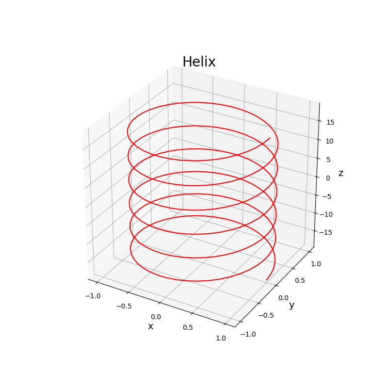
ax.plot(x, y, z, color = "red")
plt.show()
出力は以下のとおり、動かないけど似たような図が得られました。
あとは、動かせばいいということで、アニメーションを探します。
簡単に見つかるのは、matplotlib.orgのAn animated plot in 3D.が見つかりますが、以下でより近いものが見つかりました。
・Sin-Cos-tのアニメーション
【参考】
3D animation using matplotlib
これは、ほぼ答えになりそうです。
from matplotlib import pyplot as plt
import numpy as np
import mpl_toolkits.mplot3d.axes3d as p3
from matplotlib import animation

fig = plt.figure()
ax = p3.Axes3D(fig)

def gen(n):
    phi = 0
    while phi < 2*np.pi:
        yield np.array([np.cos(phi), np.sin(phi), phi])
        phi += 2*np.pi/n

def update(num, data, line):
    line.set_data(data[:2, :num])
    line.set_3d_properties(data[2, :num])

N = 100
data = np.array(list(gen(N))).T
line, = ax.plot(data[0, 0:1], data[1, 0:1], data[2, 0:1])
# Setting the axes properties
ax.set_xlim3d([-1.0, 1.0])
ax.set_xlabel('X')
ax.set_ylim3d([-1.0, 1.0])
ax.set_ylabel('Y')
ax.set_zlim3d([0.0, 10.0])
ax.set_zlabel('Z')
ani = animation.FuncAnimation(fig, update, N, fargs=(data, line), interval=10000/N, blit=False)
# ani.save('matplot003.gif', writer='imagemagick')
plt.show()
ところが、3つのアニメーションを描こうとすると、以下のようになります。
aniy = animation.FuncAnimation(fig, update, N, fargs=(datay, liney), interval=10000/N, blit=False)
anix = animation.FuncAnimation(fig, update, N, fargs=(datax, linex), interval=10000/N, blit=False)
aniz = animation.FuncAnimation(fig, update, N, fargs=(dataxy, linexy), interval=10000/N, blit=False)
この方式だと、絵的には似たようなアニメーションが得られますが、この3つのアニメーションをまとめて保存する方法が思いつきません。
・update()関数を直接呼んで描画する
以下のようにそれぞれをplt.pause(0.001)でまとめてプロットし、その図を保存することとしました。最後にそれらの図から、gif_animationを生成することとしました。
frames =100
s=180
for n in range(frames):
    s+=1
    num = s%800+200
    update(num,datax,linex)
    update(num,datay,liney)
    update(num,dataz,linez)
    plt.pause(0.001)
    plt.savefig('./sin_wave/'+str(n)+'.png'.format(elev, azim))

from PIL import Image,ImageFilter
images = []
for n in range(frames):
    exec('a'+str(n)+'=Image.open("./sin_wave/'+str(n)+'.png")')
    images.append(eval('a'+str(n)))
images[0].save('./sin_wave/sin_wave_el{}_az{}.gif'.format(elev, azim),
               save_all=True,
               append_images=images[1:],
               duration=100,
               loop=0)
そして、以下のコードのようにline.set_data(data[:2,num-200 :num])とnum = s%800+200により描画範囲を限定することにより、結果は所望のものに近づきました。
from matplotlib import pyplot as plt
import numpy as np
import mpl_toolkits.mplot3d.axes3d as p3
from matplotlib import animation

fig = plt.figure()
ax = p3.Axes3D(fig)

def genxy(n,fx,fy,fxc=0,fyc=0):
    phi = 0
    sk = 0
    while phi < 360:
        yield np.array([fx*np.cos(phi)+fxc, fy*np.sin(phi)+fyc,phi])
        phi += 36*5/n

def update(num, data, line):
    line.set_data(data[:2,num-200 :num]) #描画区間を制限する
    line.set_3d_properties(data[2,num-200 :num])

N = 960
datay = np.array(list(genxy(N,fx=0,fy=1,fxc=-2,fyc=0))).T
liney, = ax.plot(datay[0, 0:1], datay[1, 0:1], datay[2, 0:1])
datax = np.array(list(genxy(N,fx=1,fy=0,fxc=0,fyc=2))).T
linex, = ax.plot(datax[0, 0:1], datax[1, 0:1], datax[2, 0:1])
dataz = np.array(list(genxy(N,fx=1,fy=1,fxc=0,fyc=0))).T
linez, = ax.plot(dataz[0, 0:1], dataz[1, 0:1], dataz[2, 0:1])

# Setting the axes properties
ax.set_xlim3d([-2.0,2.0])
ax.set_xlabel('X')

ax.set_ylim3d([-2.0, 2.0])
ax.set_ylabel('Y')

ax.set_zlim3d([36.0, 80.])
ax.set_zlabel('Z')

frames =36
s=180
for n in range(frames):
    s+=1
    num = s%800+200
    update(num,datax,linex)
    update(num,datay,liney)
    update(num,dataz,linez)
    plt.pause(0.001)
    plt.savefig('./sin_wave/'+str(n)+'.png'.format(0, 0))

from PIL import Image,ImageFilter
images = []
for n in range(frames):
    exec('a'+str(n)+'=Image.open("./sin_wave/'+str(n)+'.png")')
    images.append(eval('a'+str(n)))
images[0].save('./sin_wave/sin_wave_el{}_az{}.gif'.format(0, 0),
               save_all=True,
               append_images=images[1:],
               duration=100,
               loop=0)
・Z軸をずらす
update()関数を以下のように書き換えて、Z軸をずらすことにします。
これによって、画像のZ軸方向は同じ位置に描画されるようになりました。
ここで軸の表示も消去します。
※因みに、Z軸の目盛も消したいところですが、最後まで消せませんでした
def update(num, data, line):
    line.set_data(data[:2,num-200 :num])
    line.set_3d_properties(data[2,num-200 :num])
    ax.set_zlim3d([0+data[2,num-200], 34+data[2,num-200]])
    ax.set_zticklabels([])
    ax.grid(False)
・図形の回転
さて、あとは座標軸をあの配置に持っていければとりあえずの完成です。
が、これが難しかったのです。
まず、軸の回転は以下で行えます。
以下では初期値の絵を軸を変えて出力しています。
for elev in range(0,360,10): #仰角の変更
    for azim in range(-180,180,5): #方位角の変更
        ax.view_init(elev, azim) #ここで座標軸の向きを調整
        frames =1  #34
        s=180
        for n in range(1): #frames
            s+=1
            num = s%800+200
            update(num,datax,linex)
            update(num,datay,liney)
            update(num,dataz,linez)
            plt.pause(0.001)
            plt.savefig('./sin_wave/'+str(n)+'{}{}.png'.format(elev, azim))
結果、あの配置は得られませんでした。
イマジネーションが足りないのですね。
上記の角度範囲以外が思いつきません。
しかし、X-Y-Zの軸見出しを変更することを思いつきました。
yield np.array([phi,fx*np.cos(phi)+fxc, fy*np.sin(phi)+fyc])
としています。
つまり、軸見出しを変更すれば螺旋が横に寝てくれます。
ということで、以下のコードにたどり着きました。
from matplotlib import pyplot as plt
import numpy as np
import mpl_toolkits.mplot3d.axes3d as p3
from matplotlib import animation

fig = plt.figure()
ax = p3.Axes3D(fig)

def genxy(n,fx,fy,fxc=0,fyc=0):
    phi = 0
    while phi < 360:
        yield np.array([phi,fx*np.cos(phi)+fxc, fy*np.sin(phi)+fyc])
        phi += 36*5/n

def update(num, data, line):
    line.set_data(data[:2,num-200 :num])
    line.set_3d_properties(data[2,num-200 :num])
    ax.set_xlim3d([0+data[0,num-200], 36+data[0,num-200]])
    ax.set_xticklabels([])
    ax.grid(False)

N = 960
datay = np.array(list(genxy(N,fx=0,fy=1,fxc=-2,fyc=0))).T
liney, = ax.plot(datay[0, 0:1], datay[1, 0:1], datay[2, 0:1])
datax = np.array(list(genxy(N,fx=1,fy=0,fxc=0,fyc=-2))).T
linex, = ax.plot(datax[0, 0:1], datax[1, 0:1], datax[2, 0:1])
dataz = np.array(list(genxy(N,fx=1,fy=1,fxc=0,fyc=0))).T
linez, = ax.plot(dataz[0, 0:1], dataz[1, 0:1], dataz[2, 0:1])

# Setting the axes properties
ax.set_xlim3d([20, 70.0])
ax.set_xlabel('Z')
ax.set_ylim3d([-2.0, 2.0])
ax.set_ylabel('X')
ax.set_zlim3d([-2.0, 2.0])
ax.set_zlabel('Y')

elev=20.
azim=35.
ax.view_init(elev, azim)

frames =100
s=180
for n in range(frames): #frames
    s+=1
    num = s%800+200
    update(num,datax,linex)
    update(num,datay,liney)
    update(num,dataz,linez)
    plt.pause(0.001)
    plt.savefig('./sin_wave/'+str(n)+'.png'.format(elev, azim))

from PIL import Image,ImageFilter
images = []
for n in range(frames):
    exec('a'+str(n)+'=Image.open("./sin_wave/'+str(n)+'.png")')
    images.append(eval('a'+str(n)))
images[0].save('./sin_wave/sin_wave_el{}_az{}.gif'.format(elev, azim),
               save_all=True,
               append_images=images[1:],
               duration=100,
               loop=0)
こうして、最初に掲載した3Dアニメーションが出力できました。
・3Dリサジュー図形
もっとも、本来やりたかったのは3Dリサジュー図形なので、いくつかやってみます。
以下を変更して滑らかに繋がるようにframes=200を変更すれば出来ます。
yield np.array([phi,fx*np.cos(3*phi/2)+fxc, fy*np.sin(2*phi/3)+fyc])
X : Y = 1 : 2
X : Y = 1/2 : 2/3
X : Y = 3/2 : 2/3
まとめ
・Sin-Cos-tの3Dアニメーションを描いて見た
・3Dアニメーションが描けるようになった
・3Dリサジュー図形を描いてみた
※二次元リサジュー図形(上記のXY面への写像)はググってみてください
おまけ
完成版
原点にリサジュー図形を描画するように改良しました
3d_animation_Risajyu/3D_animation_risajyu.py
point追加