K-meansクラスタリングは、簡単に云うと「適当な乱数で生成された初期値から円(その次元を持つ境界が等距離な多様体)を描いてその中に入る点をその中心(重心)に属する」という考え方でクラスタリングしている。
つまり、以下の式の最適化問題である。
given\left \{
 \begin{array}{l}
cluster\ No.:\ k\\
data\ No.:\ n\\
 \end{array}
 \right.\\
 {arg\,min} _{V_{1},\dotsc ,V_{k}}\sum _{i=1}^{n}\min _{j}\left\|x_{i}-V_{j}\right\|^{2}
実際のアルゴリズムは参考によれば、以下のとおりである。
(以下、Wikipediaから引用)
「k-平均法は、一般には以下のような流れで実装される[5][6]。データの数を $n$、クラスタの数を $k$ としておく。
- 各データ $x_i$ $(i=1,...,n)$ に対してランダムにクラスタを割り振る。
- 割り振ったデータをもとに各クラスタの中心 $V_j$ $(j=1,...,k)$ を計算する。計算は通常割り当てられたデータの各要素の算術平均が使用されるが、必須ではない。
- 各 $x_i$ と各 $V_j$ との距離を求め、 $x_i$ を最も近い中心のクラスタに割り当て直す。
- 上記の処理で全ての $x_i$ のクラスタの割り当てが変化しなかった場合、あるいは変化量が事前に設定した一定の閾値を下回った場合に、収束したと判断して処理を終了する。そうでない場合は新しく割り振られたクラスタから $V_j$ を再計算して上記の処理を繰り返す。」
【参考】
・k平均法@wikipedia
今回は、このアルゴリズムだとクラスタリング出来ないケースがあるということで、それをどうするというところまで書きたいと思う。
やったこと
・moonsやドーナツ型はだめらしい
・moonsやcirclesを分類できるspectral clustering
・moonsやドーナツ型はだめらしいが、。。
とにかくやってみる
import matplotlib.pyplot as plt
from sklearn.cluster import KMeans # K-means クラスタリングをおこなう
from sklearn.decomposition import PCA #主成分分析器
import numpy as np
from sklearn.datasets import make_moons
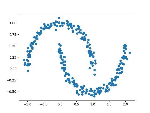
まず、moonsを生成する。
N =300
noise=0.05
X, y = make_moons(N,
                  noise=noise,
                 random_state=0)
plt.scatter(X[:,0],X[:,1])
plt.pause(1)
plt.close()
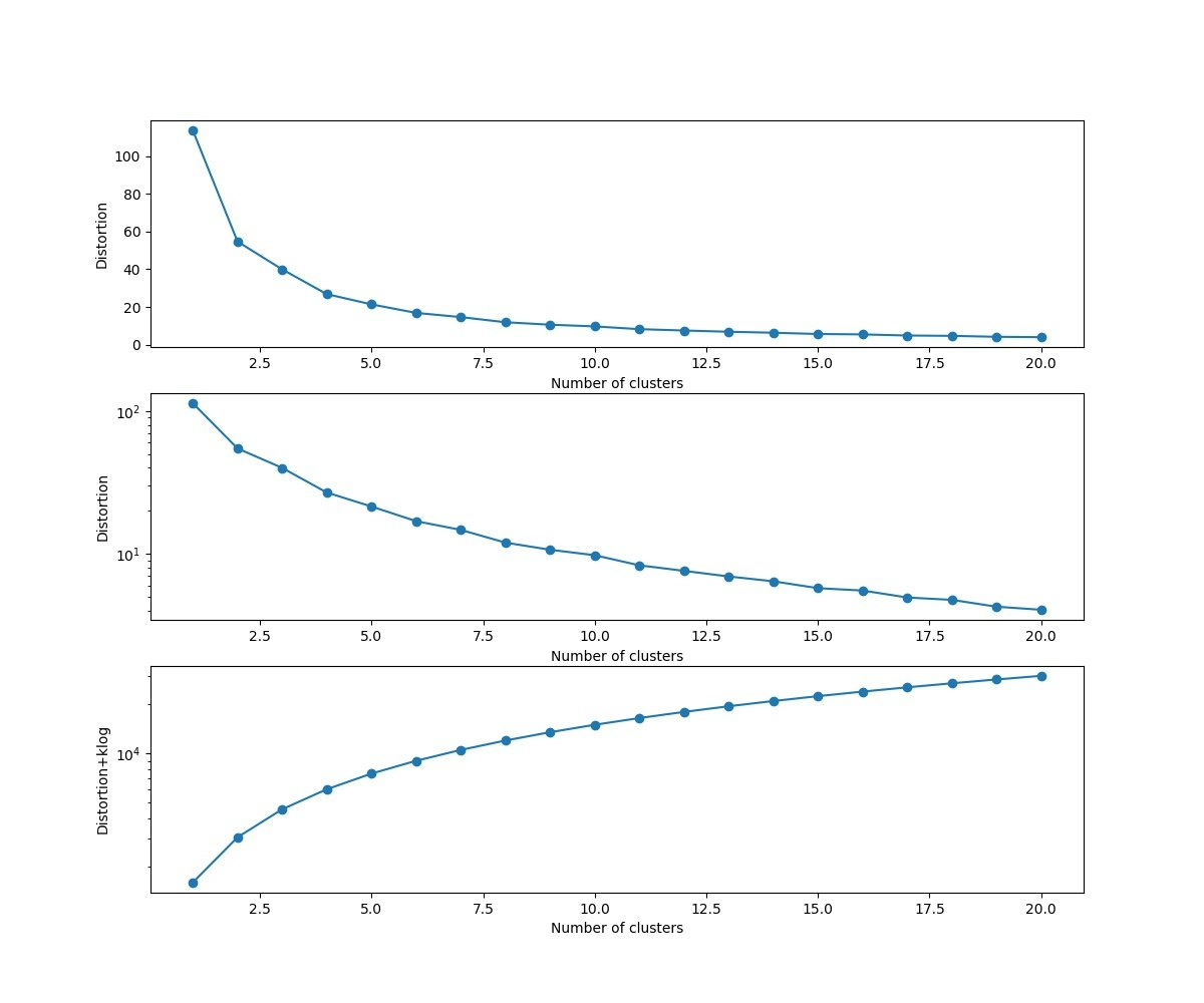
まず、Kを変えてDistorsionの変化を見る。
distortions = []
distortions1 = []
for i  in range(1,21):                # 1~20クラスタまで一気に計算
    km = KMeans(n_clusters=i,
                init='k-means++',     # k-means++法によりクラスタ中心を選択
                n_init=10,
                max_iter=300,
                random_state=0)
    km.fit(X)                # クラスタリングの計算を実行 #df.iloc[:, 1:]
    distortions.append(km.inertia_)       # km.fitするとkm.inertia_が得られる
    UF = km.inertia_ + i*np.log(20)*5e2   # km.inertia_ + kln(size)
    distortions1.append(UF)
fig=plt.figure(figsize=(12, 10))
ax1 = fig.add_subplot(311)
ax2 = fig.add_subplot(312)
ax3 = fig.add_subplot(313)
ax1.plot(range(1,21),distortions,marker='o')
ax1.set_xlabel('Number of clusters')
ax1.set_ylabel('Distortion')
# ax1.yscale('log')
ax2.plot(range(1,21),distortions,marker='o')
ax2.set_xlabel('Number of clusters')
ax2.set_ylabel('Distortion')
ax2.set_yscale('log')
ax3.plot(range(1,21),distortions1,marker='o')
ax3.set_xlabel('Number of clusters')
ax3.set_ylabel('Distortion+klog')
ax3.set_yscale('log')
plt.pause(1)
plt.savefig('k-means/moons/moons'+str(noise)+'_Distortion.jpg')
plt.close()
moonsではDistorsionの図はだらだらしていて最適なkは見つからない。
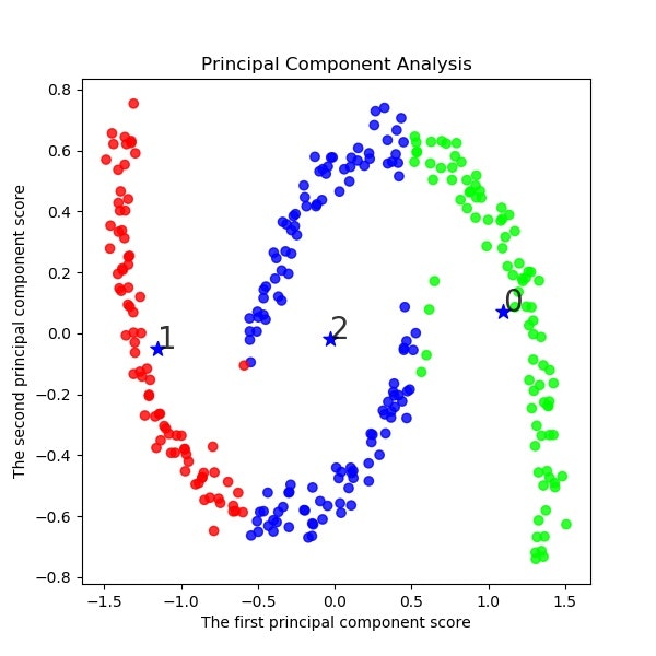
以下でK-meansクラスタリングする。ここでは初期値をinit='k-means++'として工夫している。
s=2
km = KMeans(n_clusters=s,
                init='k-means++',     # k-means++法によりクラスタ中心を選択
                n_init=10,
                max_iter=300,
                random_state=0)
y_km=km.fit_predict(X)  #df.iloc[:, 1:]
# この例では s個のグループに分割 (メルセンヌツイスターの乱数の種を 10 とする)
kmeans_model = KMeans(n_clusters=s, random_state=10).fit(X)  #df.iloc[:, 1:]
# 分類結果のラベルを取得する
labels = kmeans_model.labels_
print(labels)     ##################  print(labels) ###################
# それぞれに与える色を決める。
color_codes = {
    0:'#00FF00', 1:'#FF0000', 2:'#0000FF', 3:'#00FFFF' , 4:'#00FF77', 5:'#f0FF00', 6:'#FF06F0', 7:'#0070FF', 8:'#FFF444' , 9:'#077777',
    10:'#111111',11:'#222222',12:'#333333', 13:'#444444',14:'#555555',15:'#66FF00', 16:'#FF7777', 17:'#0000FF', 18:'#00FFFF',19:'#007777'}
# サンプル毎に色を与える。
colors = [color_codes[x] for x in labels]
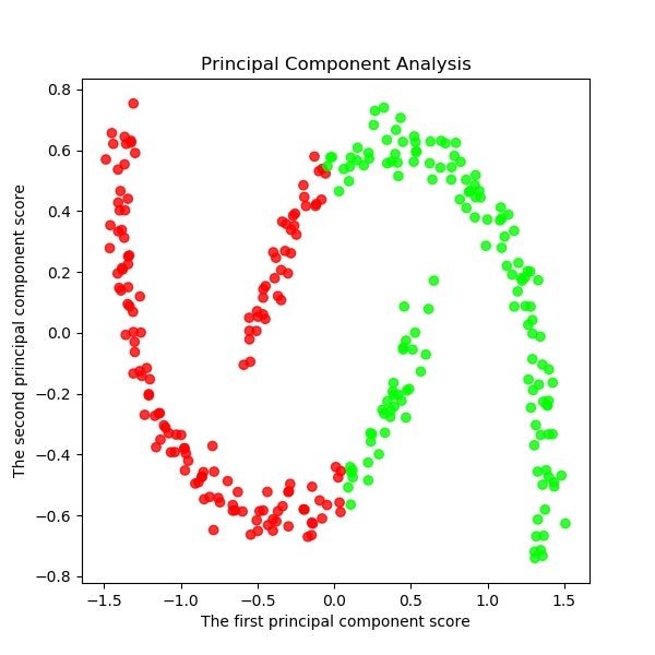
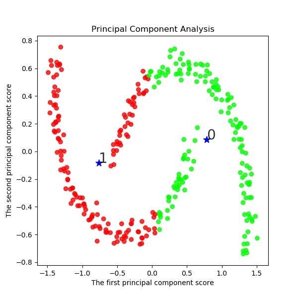
以下でPCA主成分分析を実施する。
# 主成分分析の実行
pca = PCA()
pca.fit(X) #df.iloc[:, 1:]
PCA(copy=True, n_components=None, whiten=False)
# データを主成分空間に写像 = 次元圧縮
feature = pca.transform(X) #df.iloc[:, 1:]
x,y = feature[:, 0], feature[:, 1]
print(x,y)
X=np.c_[x,y]
plt.figure(figsize=(6, 6))
plt.title("Principal Component Analysis")
plt.xlabel("The first principal component score")
plt.ylabel("The second principal component score")
plt.savefig('k-means/moons/pca/moons'+str(noise)+'_PCA12_plotSn'+str(s)+'.jpg')
plt.pause(1)
plt.close()
結果は予想通り、右と左に色分けしている。
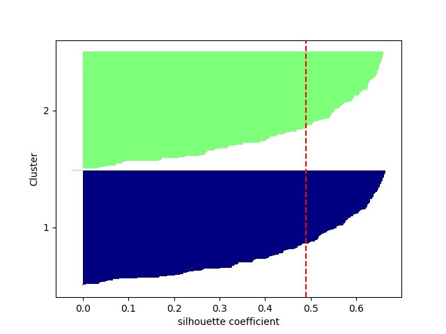
from sklearn.metrics import silhouette_samples
from matplotlib import cm

cluster_labels = np.unique(y_km)       # y_kmの要素の中で重複を無くす s=6 ⇒ [0 1 2 3 4 5]
n_clusters=cluster_labels.shape[0]     # 配列の長さを返す。つまりここでは n_clustersで指定したsとなる

# シルエット係数を計算
silhouette_vals = silhouette_samples(X,y_km,metric='euclidean')  # サンプルデータ, クラスター番号、ユークリッド距離でシルエット係数計算 df.iloc[:, 1:]
y_ax_lower, y_ax_upper= 0,0
yticks = []

for i,c in enumerate(cluster_labels):
        c_silhouette_vals = silhouette_vals[y_km==c]         c_silhouette_vals.sort()
        y_ax_upper += len(c_silhouette_vals)
        color = cm.jet(float(i)/n_clusters)
        plt.barh(range(y_ax_lower,y_ax_upper),
                         c_silhouette_vals,
                         height=1.0,
                         edgecolor='none',
                         color=color)
        yticks.append((y_ax_lower+y_ax_upper)/2)
        y_ax_lower += len(c_silhouette_vals)
silhouette_avg = np.mean(silhouette_vals)                 # シルエット係数の平均値
plt.axvline(silhouette_avg,color="red",linestyle="--")    # 係数の平均値に破線を引く
plt.yticks(yticks,cluster_labels + 1)                     # クラスタレベルを表示
plt.ylabel('Cluster')
plt.xlabel('silhouette coefficient')
plt.savefig('k-means/moons/moons'+str(noise)+'_silhouette_avg'+str(s)+'.jpg')
plt.pause(1)
plt.close()
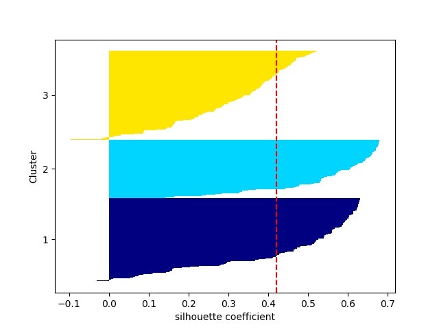
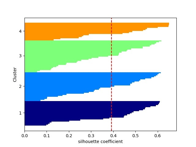
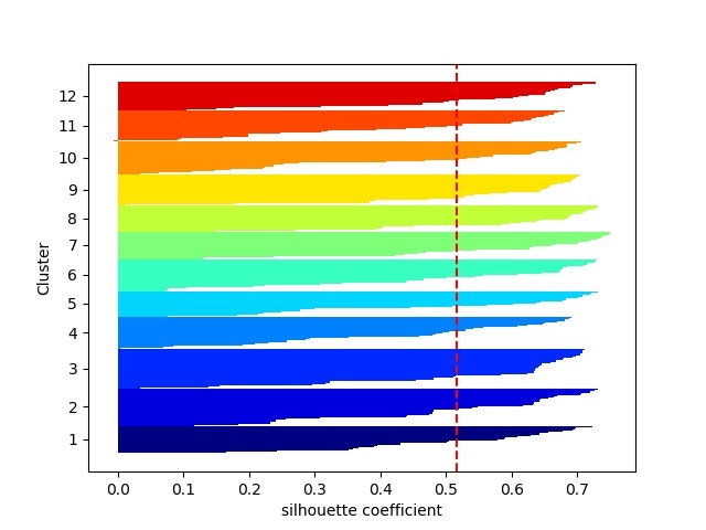
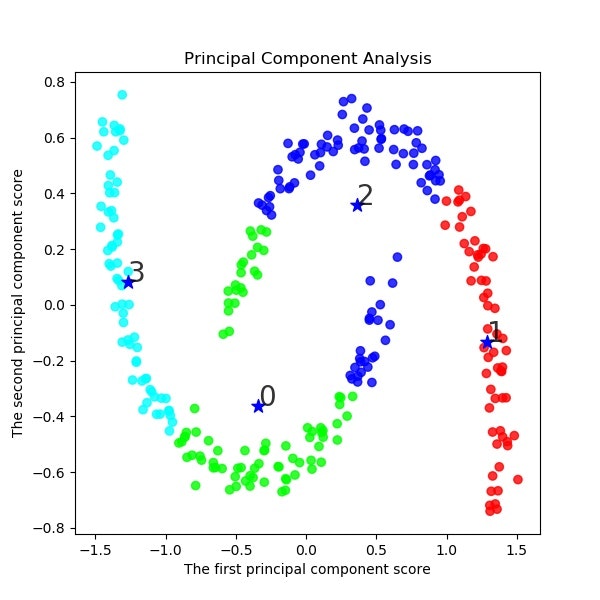
シルエット係数は以下のようになる。クラス数を増やしてもmoonsの場合はある意味バランスはいい
。。。
# この例では s つのグループに分割 (メルセンヌツイスターの乱数の種を 10 とする)
kmeans_model = KMeans(n_clusters=s, random_state=10).fit(X)
# 分類結果のラベルを取得する
labels = np.unique(kmeans_model.labels_) #kmeans_model.labels_ cluster_labels
# 分類結果を確認
print(labels) ################# print(labels) ############
# サンプル毎に色を与える。
colors = [color_codes[x] for x in kmeans_model.labels_]
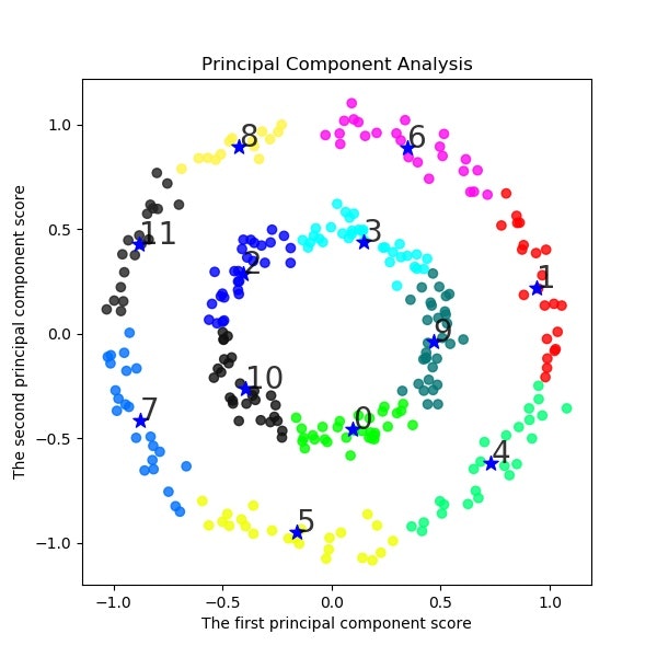
# 第一主成分と第二主成分でプロットする
plt.figure(figsize=(6, 6))
for kx, ky, name in zip(kmeans_model.cluster_centers_[:,0], kmeans_model.cluster_centers_[:,1], labels):
plt.text(kx, ky, name, alpha=0.8, size=20)
plt.scatter(x, y, alpha=0.8, color=colors)
plt.scatter(kmeans_model.cluster_centers_[:,0], kmeans_model.cluster_centers_[:,1], c = "b", marker = "*", s = 100)
plt.title("Principal Component Analysis")
plt.xlabel("The first principal component score")
plt.ylabel("The second principal component score")
plt.savefig('k-means/moons/pca/moons'+str(noise)+'_PCA12_plotn'+str(s)+'.jpg')
plt.pause(1)
plt.close()
。。。

11クラスだと8の上辺のところが4に属していてまずいような気がする。
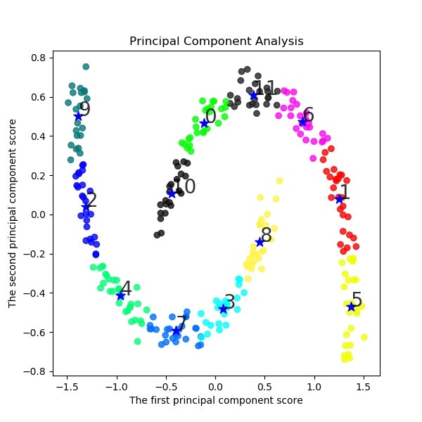
12クラス使うと、一応クラスタリング出来たことになるが、人の目だと2クラスで分類できるので、結果は大きく異なっている。
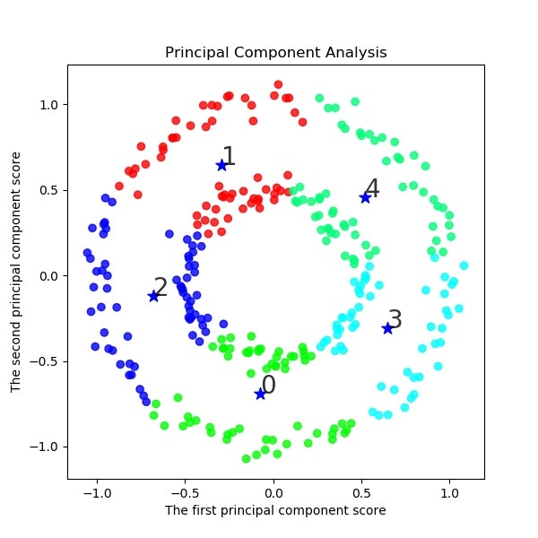
一方、同じようにドーナツ型の場合も以下のような結果となる。
コードは以下の変更をするだけである。
from sklearn.datasets import make_moons, make_circles

N =300
noise=0.05
X, z = make_circles(n_samples=N, factor=.5, noise=noise)
# X, y = make_moons(N, noise=noise, random_state=0)
結果はmoonsとほぼ同じく、クラスタ間の距離が同心円の内外の距離より小さくなるとクラスタリングが成功するが、やはり人間の目の感覚とは異なる分類となっている。
・moonsやcirclesを分類できるspectral clustering
spectral clusteringだとmoonsもcirclesも簡単にクラスタリングしてくれる。。。
【参考】
・sklearn.cluster.SpectralClustering
実際コードで動かしてみると以下のとおり、選べるパラメーターは以下のとおりですが、初心者が簡単に選べるのは、。assign_labels : {‘kmeans’, ‘discretize’}と affinity : {‘rbf’, ‘nearest_neighbors’}あたりかなと思います。
assign_labels : {‘kmeans’, ‘discretize’}, default: ‘kmeans’
affinity : string, array-like or callable, default ‘rbf’
 If a string, this may be one of ‘nearest_neighbors’, ‘precomputed’, ‘rbf’ or one of the kernels supported by sklearn.metrics.pairwise_kernels.
使うものは以下のとおり
from sklearn.cluster import SpectralClustering
import numpy as np
import matplotlib.pyplot as plt #プロット用のライブラリを利用
from sklearn.datasets import make_moons, make_circles
データは上と同じものを選びます。
N =300
noise=0.05
# X, z = make_circles(n_samples=N, factor=.5, noise=noise)
X, z = make_moons(N, noise=noise, random_state=0)
plt.scatter(X[:,0],X[:,1])
plt.title("original")
plt.pause(1)
plt.close()
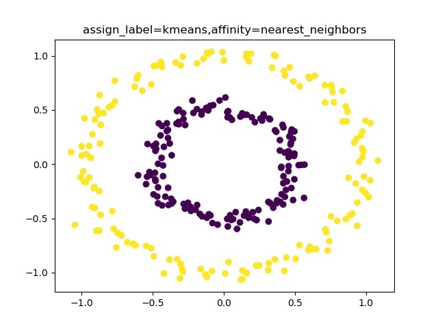
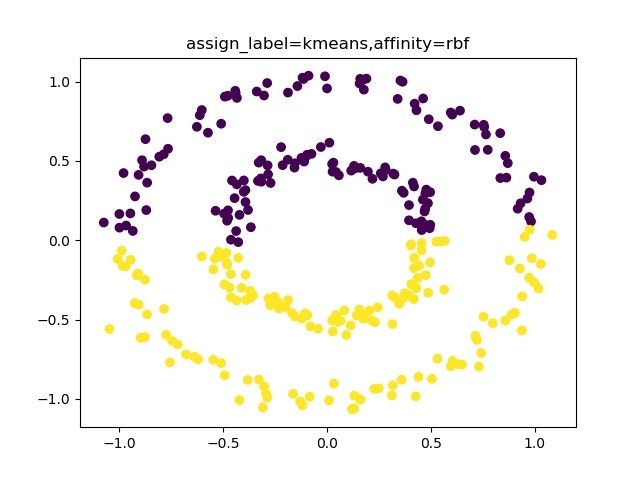
4種類の組み合わせを以下のように明示的に実施します。
s=2
lists_Alabel={"discretize","kmeans"}
lists_Affinity={"nearest_neighbors","rbf"}
for l in lists_Alabel:
    for af in lists_Affinity:
        clustering = SpectralClustering(n_clusters=s, assign_labels=l, random_state=0,affinity=af).fit(X)
        print(clustering.labels_)
        plt.scatter(X[:,0],X[:,1], c=clustering.labels_)
        plt.title("assign_label={},affinity={}".format(l,af))
        plt.pause(1)
        plt.savefig('k-means/spectral/moons'+str(l)+str(af)+'_PCA'+str(s)+'.jpg')
        plt.close()
実際動かしてみると、いつもクラスタリング出来るわけではなく、affinity : {‘nearest_neighbors’}のときに人の目で見たようにクラスタリングしてくれることが分かります。


まとめ
・K-meansのちょっと理論にて、クラスター重心でクラスタリングしていることを見た
・その結果、moonsやcirclesのような距離が複雑な分布を持つ場合のクラスタリングは苦手であることが分かった
・spectral clusteringでは、属性としてaffinity="nearestneighbers"を選ぶことにより、単純な距離よりもつながりでクラスターを見ることにより、上記の複雑な場合もクラスタリングできることが分かった
・spectral-clusteringの理論や多変量への応用については次回記載したいと思う